What is a p value, and how it relates to error rates?
The p-value might seem simple at first, but the definition tends to confuse people. Formally, the p-value is the probability of obtaining a result at least as extreme as the result observed, when the null hypothesis is true (i.e. when there is no effect, or no difference). Less formally, if we start off thinking the null is true (no effect), how surprised are we by the result? If we’re sufficiently surprised, we reject the null and go with the alternative hypothesis.
In practice, imagine we ran many A/A experiments, where both groups receive no treatment (i.e. we know the null is true, there is no effect). This tells us the range of possible values to expect under the null. Comparing an observed treatment effect to that distribution, we can calculate how often we observe an effect at least as extreme as that (i.e. the p-value). If the p-value is very low, it’s very uncommon to see a result like this when the null is true, so we take it as evidence towards the null being false.
Keep in mind we haven’t proven anything, but rather use our level of ‘surprise’ to guide our decision. There is always some risk of a false positive (incorrectly rejecting the null). Therefore, depending on our risk tolerance, we should adjust our bar for ‘surprise’ accordingly and ensure we follow a scientific method.
An analogy
A useful analogy for some is the concept of ‘innocent until proven guilty’ in the legal system. If the evidence indicates the accused it guilty ‘beyond a reasonable’ they are found guilty. Otherwise, they are ‘not proven to be guilty’ or ‘not guilty’. This doesn’t mean they are not guilty, but rather there was insufficient evidence to persuade the jury/judge. Similarly, in a hypothesis test, we start by assuming the null hypothesis is true. We reject the null only if we have sufficient evidence (p less than 0.05), else we fail to reject the null. If we don’t reject the null, this doesn’t mean there isn’t an effect, but we had insufficient evidence to persuade us.
Common misunderstandings and a few points to remember:
1. Remember it’s conditioned on the null hypothesis being true
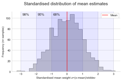
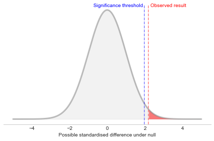
\[p value = P(\text{observed difference} \:|\: H_\text{o} true)\]Let’s say we are comparing means. We can estimate the distribution under the null with a normal or t distribution (based on CLT the distribution of the mean difference will converge to normal with large samples so long as the variance is finite). You might be familiar with the 68-95-99.7 rule, which applied here tells us 68% of the results with be within ~1 standard deviation of the mean (0, or no difference), 95% within ~2 standard deviation, and 99.7% within ~3. By setting alpha to 0.05, we want 95% of the data to be less than our absolute threshold, so we reject the null when the result is greater than or equal to +/- 1.96 standard deviations from the mean (alpha/2=0.25 or 2.5% in each tail).

Now we just need to locate where our result falls in this distribution. The p-value will simply be the area under the curve in the tail, when we cut at our observed value. From the plot, if the cut is more extreme or equal to the significance threshold, we will reject the null. Otherwise, we fail to reject the null (it could be true or not).

2. The p-value is not the probability of the null being true
Some get confused and think the p-value is the probability that the null hypothesis is true. However, as we noted above it’s conditioned on the null being true, so this is incorrect. It may help to think about the extreme case where we only run A/A experiments. In this case, the null hypothesis is true 100% of the time. Inversely, if all of our experiments are effective, then the null is true 0% of time. However, in both cases, we can still run a hypothesis test and assess the evidence based on the probability of the result, assuming that the null hypothesis is true.
To calculate the probability the null hypothesis is true, given some observed difference, we would also need the prior probability the null hypothesis is true:
\[P( H_\text{o}\:\text{true} \:|\: \text{observed difference}) = \frac{P(\text{observed difference} \:|\: H_\text{o}\:\text{true}) * P(H_\text{o}\:\text{true})}{P(\text{observed difference})}\] \[= \frac{P(H_\text{o} true)}{P(\text{observed difference})} * pvalue\]3. The inverse of the p-value (1-p) is not the probability the alternate is true
As we’re conditioning on the null being true, we are only looking at possible outcomes when the null is true. So the inverse would be the probability of a less extreme result (the rest of the distribution), again assuming the null is true. We never prove the alternate is true with a hypothesis test, but rather gather evidence against of whether it’s likely that the null is true. If it’s unlikely, we reject the null and accept the alternate.
4. The results depend on the significance level chosen
You might be wondering how small is small enough for us to conclude the null is ‘unlikely’ enough to accept the alternate? The answer is not so satisfying, we have to pre-define a threshold at which point we will reject the null. The threshold (alpha) is the false positive rate (when the null is true, how often we’ll reject the null). The smaller the threshold, the lower the false positive rate, but the larger the sample needed to detect an effect when it exists. There will always be a trade-off. A common choice is 0.05, which means we reject the null when the p-value is less than 0.05, accepting a false positive rate of 5% (i.e. 1/20 times we reject the null when it’s actually true).
Note, if you plan to test many hypotheses, you may want to decrease the significance level to correct for multiple testing. For example, let’s say you think jelly beans cause acne, and you want to test this hypothesis for 20 jelly bean colours with a FPR of 5% for each test. The chance of a False Positive across the 20 tests is not 5% but much higher. A shown below, the probability of no False Positives is 35.8%, so the probability of at least one is 64.2%.
\[P(no False Positives) = \frac{20!}{(20-0)!0!} * 0.05^0 * 0.95^(20-0) = 0.358\]A conservative adjustment is the Bonferroni correction, which divides alpha by the number of tests. E.g. for 20 tests and a FPR of 5%, the alpha for each test is 0.05/20=0.0025. In experimentation, another common approach is to set alpha for groups of metrics based on how strong our prior beliefs are, e.g. 1st order (expect to impact), 2nd order (potentially impact), and 3rd order (unlikely to be impacted). Then assign decreasing significance levels to each group (e.g. 0.05, 0.01, 0.001). This method is recommended by Kohavi et al., 2020. Similarly, another approach is to use the more exploratory metrics and segment breakdowns as inspiration only. Develop on these ideas, and then retest them in a new experiment.
5. The p-value and confidence interval always agree
If the p-value is significant, the confidence interval for the difference won’t overlap with the null (i.e. 0 if the null is no difference), and vice versa. Assuming they’re generated by the same hypothesis test, and significance level. The reason is the significance level determines the distance from the estimated effect to the upper and lower limit of the confidence interval, as well as the distance from the null to the critical regions.
Just remember, we’re looking at the confidence interval of the difference, not of each sample. If we compare the confidence interval around the estimate for each sample, it can still be significant even if they overlap.
6. One-sided p-value is half the two-sided
If the hypothesis is one-sided e.g. Ho: mean 2 <= mean 1 and Ha: mean 2 > mean 1, then we only take the probability in one-tail for the p-value (vs both tails for a two sided hypothesis like mean 1 != mean 2). That’s why the one-sided p-value is half the two-sided. However, in general a two-sided test is recommended, unless you have good reason to believe a specific direction, and you are not concerned about errors in the opposite direction.
7. False positive rate (FPR) vs false discovery rate (FDR)
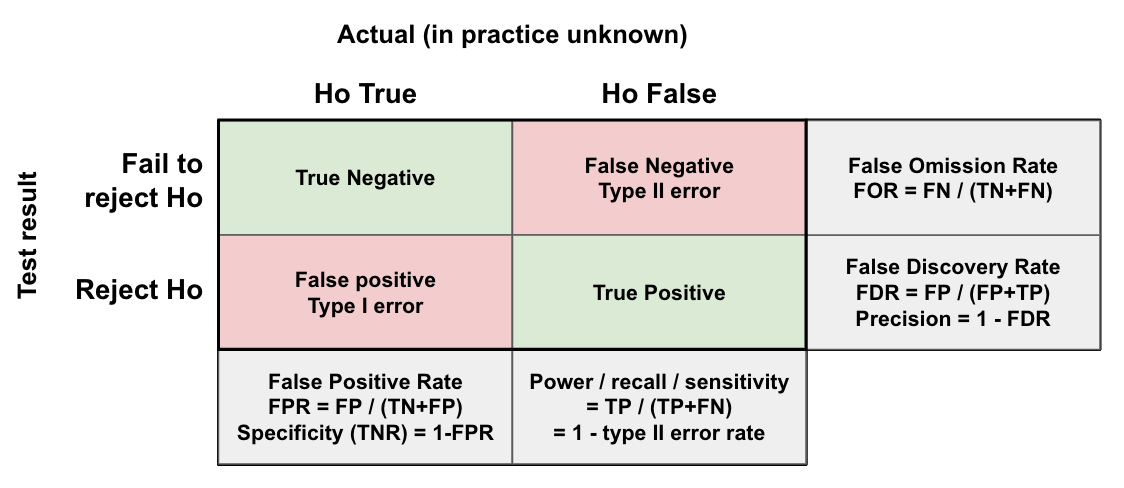
As shown below, the FPR is how often we incorrectly reject the null (False Positive), as a proportion of all the times the null is true (which we control with the significance level, alpha). However, another important measure is the false discovery rate (FDR), or what proportion of the observed positive results are false positives (which depends on the prior for Ha being true, the significance level (FPR), and power of the test).

The FDR answers the question: if our p-value is significant (<0.05 if we set alpha to 0.05), what is the chance there is really no effect and it’s just due to random chance? Imagine we are testing the effectiveness of various drugs for asthma. We have data from 1000 trials. Each experiment determined the sample size based on a FPR of 5% and power of 80%. What proportion of the drugs we approve are actually effective? This depends on the prior. Let’s consider 3 scenarios:
- Every trial is actually ineffective (Ho always true): We expect 5% (50/1000) of the trials to still pass and reject the null (FPR). As Ha is never true, we have no true positives. Therefore the FDR is 100% (50/50 of the positive results are incorrect).
- Let’s say we did a little better and now 10% of the trials are actually effective (100/1000). We expect 0.8 * 100 = 80 True Positives (20 False Negatives), and 0.05 * 900 = 45 False Positives (855 True Negatives). Therefore, the FDR = 45 / (80 + 45) = 36%.
- If we did even better and now 50% of the trials are actually effective (500/1000). With 80% power we expect 0.8500 = 400 True Positives (100 False Negatives), and with the 5% FPR we expect 0.05500 = ~25 False Positives (475 True Negatives). Therefore, the FDR is 25 / (25 + 400) = 5.89%.
These scenarios demonstrate that the better our hypotheses are (i.e. the more likely they are to actually be effective), then the lower our False Discovery Rate is (holding the FPR and power constant). If we are just testing lots of random changes with little thought, it’s possible that a high proportion of the trials we approve (or product changes we make) are actually ineffective and likely not reproducible. To reduce the FDR we can increase the sample size (so power increases), or decrease the significance level (as with the corrections before for multiple testing). We can also work incrementally, improving on ideas that appear effective (significant), so that we also check the reproducibility. Finally, the biggest lever is the quality of the hypotheses, which we can try improve by using other sources of information such as user research, historical data, and external data in our development process.
Final thoughts
- One reason for the misunderstandings is that the p-value doesn’t deliver what most people really want to know: the probability the hypothesis is correct. For that we would need to consider the prior probabilities.
- It’s also important to use common sense, and consider the p-value in combination with other information (e.g. other sources of evidence). A low p-value doesn’t mean the effect is large or even meaningful in practice. E.g. If eating an apple a day reduces the length of a pregnancy by 4 hours on average, is this meaningful? Most likely the women would not have even noticed. When you’re working with very large samples, even small differences will be statistically significant.
- The more we do to improve our hypotheses before testing, the better (lower) our false discovery rate will be. As we saw above, the false discovery rate can be much higher than the false positive rate if the quality of hypotheses is low. This is where analytics and user research can really help teams to identify and focus on the most promising changes.
- While a high FDR may seem relatively harmless in a business setting, it can result in a lot of wasted time working in the wrong direction. E.g. If you reward team’s based on the number of successful experiments, a team that runs many low quality experiments could appear more successful and get more investment.
- A counter argument is that we may care more about False Negatives (missed opportunities) than we do about False positives (false alarms). By reducing the type I errors, we increase the type II errors (i.e. by decreasing the significance level, we can only detect larger effects, all else equal). In some settings, a relatively high significance level like 0.1 is used for exactly this reason.
- The p-value can easily be abused so it gets a bad reputation. If we run many tests, we’ll eventually get a false positive. See here for a good explanation of the different kinds of p-hacking many of us are guilty of. However, again, the counter argument to this article is that in some business settings we care more about the False Negatives. In this case, we should follow up with an experiment, or other ways of testing the hypothesis to ensure it’s reproducible.
References: