April 11, 2021

Statistical power: concept and calculations

The statistical power of a test is simply the chance of detecting an effect, when one exists. The concept may be more familiar in the context of a medical test. For example, let’s say the power of a diabetes test is 80%. This means that if you have diabetes, there’s an 80% chance you will test positive (True Positive), and a 20% chance you will incorrectly test negative (False Negative). However, there’s also likely a small chance that you test positive even if you don’t have diabetes (False Positive). When designing the test, we have to balance the risk of False Negatives (e.g. delaying treatment), with the cost of False Positives (e.g. giving unnecessary treatment and medications). Though a bit less extreme, the same is true in business experiments: False Negatives are missed opportunities for business impact, while False Positives could lead us to wasting time working in the wrong direction. The goal of the power analysis is to help us make these trade-offs while determining the sample size required (i.e. how long we need to run the experiment).

Power analysis

A power analysis tells us the sample size required for a given power, significance level, and minimum detectable effect. We are essentially just re-arranging the formula for the statistical test to instead output the sample size for the given inputs. By varying the significance level and power we can trade-off the False Positives (type I error) and False Negatives (type II error) respectively, as discussed above. It’s important that we do this step before the experiment, as changing the requirements mid experiment increases the False Positive Rate, and an under-powered experiment (e.g. values less than 50%) is unlikely to detect an effect even if one exists.

Components

The output:

Sample size: How many total observations are required for the test. We can divide this by the average number of new observations per day to get the runtime. Keep in mind these should be unique observations, so repeat visitors are only counted once. For example, if you’re randomising visitors, count each unique visitor only on the first day they would have been seen to simulate the experiment setting (which will lower your expected number on later days if you have many repeat visitors).

The inputs:

Statistical power: The chance of detecting an effect when one actually exits. This is the inverse of the type II error rate (i.e. False Negatives as a proportion of those where Ho is False). The higher the power, the larger the sample size needed. A common choice is 0.8 (80%), meaning there’s a 20% chance of a False Negative when there is actually an effect (Ho False).
Significance level: The chance of incorrectly detecting an effect (rejecting Ho) when Ho is True (i.e. the False Positive Rate (FPR), or type I error rate). The lower the significance level, the larger the sample size needs to be. The most common value chosen is 0.05 (5% FPR), but this is somewhat arbitrary. Note, decreasing the significance level to decrease the FPR will also reduce the power, all else equal (as we increase False Negatives by making the significance cutoff tougher).
Minimum detectable effect: The minimum effect that would be meaningful for this particular change. The smaller the effect you want to be able to detect, the larger the sample size will need to be (required sample approaches infinity as the effect approaches 0). This is often a tough one for those new to experimentation, but a necessary step. One approach is to consider the costs of implementing the change, e.g. how big does the effect need to be for it to be worthwhile? Or try thinking about possible results, e.g. if it’s a 1%/2%/5% change, what would we do?
Sampling ratio: The ratio of observations in control vs variant. The optimal ratio in terms of sample size is 1:1 (i.e. a 50%/50% split in observations). Deviations in either direction increase the required sample size. However, sometimes due to the cost or risk of exposing people to the treatment, a lower proportion of observations are assigned to the variant group. In this case, it’s best to put the ‘spare’ observations in the control group to maximise power (as opposed to excluding them to get a 50/50 split). I’ll demonstrate this below with an example.

Sampling ratio example

Let’s say we have 1000 visitors per day, the base mean is 5 (muA=5), standard deviation = 8, and we want a minimum detectable effect of 0.5 (muB=5.5). We’ve been told we can only give the treatment to 10%, so we have 2 options:

1) Split 50/50: put 10% in control and 10% in variant, giving us 200 visitors per day (20%). Plugging in our values with a sampling ratio of 1 (nA/nB), we will need a total of 8022 visitors (4011 in each group). With 200 visitors per day, our runtime is 8,022 / 200 = 40 days.
2) Split 90/10: put 10% in variant and the remaining 90% in control, giving us the full 1000 visitors per day. Due to the uneven split (ratio=nA/nB=9/1=9), we now need a total of 22,280 visitors (nA=20,052 and nB=2228). However, despite the higher total, as we have a larger daily sample, we only need a runtime of 22,280 / 1000 = 22 days.

Sample size calculator used for the above.

An analogy

An analogy often used to help non-technical stakeholders understand power is the fishing net. A net with large holes is cheaper to make, but can only catch large fish (i.e. large effects). The net with small holes takes more time and money, but can catch smaller fish (i.e. small to medium effects). So the smaller the effect we want to detect, the longer the runtime will need to be.

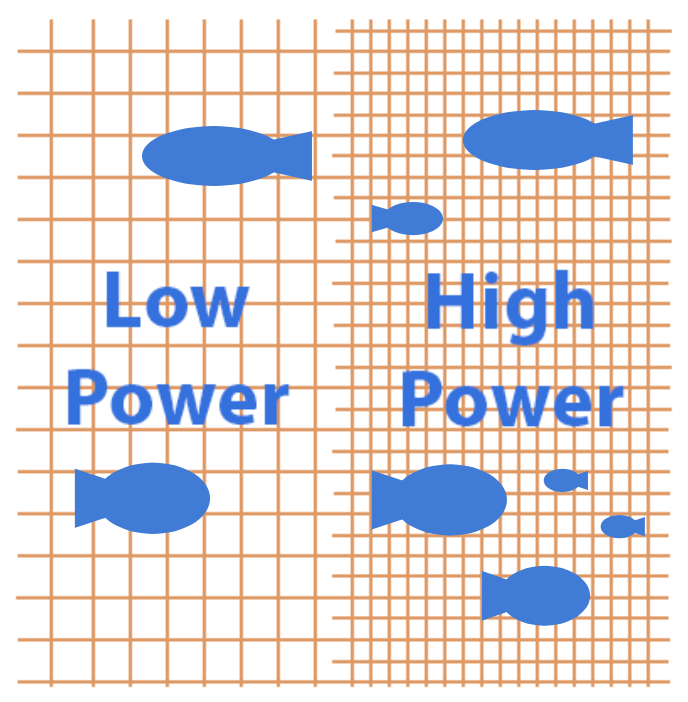Fishing net analogy Source: Altered version of image from here.

Why low power = questionable results

While it is still possible to detect an effect when one exists with low power (e.g. 20% power means we will correctly detect the effect 20% of the time), this can result in a high False Discovery Rate (FDR). The FDR measures the proportion of the ‘positive’ tests (i.e. p-value is significant), that are actually false positives. Decreasing the power increases the FDR as the number of True Positives decreases while the number of False Positives remains the same. Therefore, many of our tests which we think are effective, may not be.

Confusion Matrix

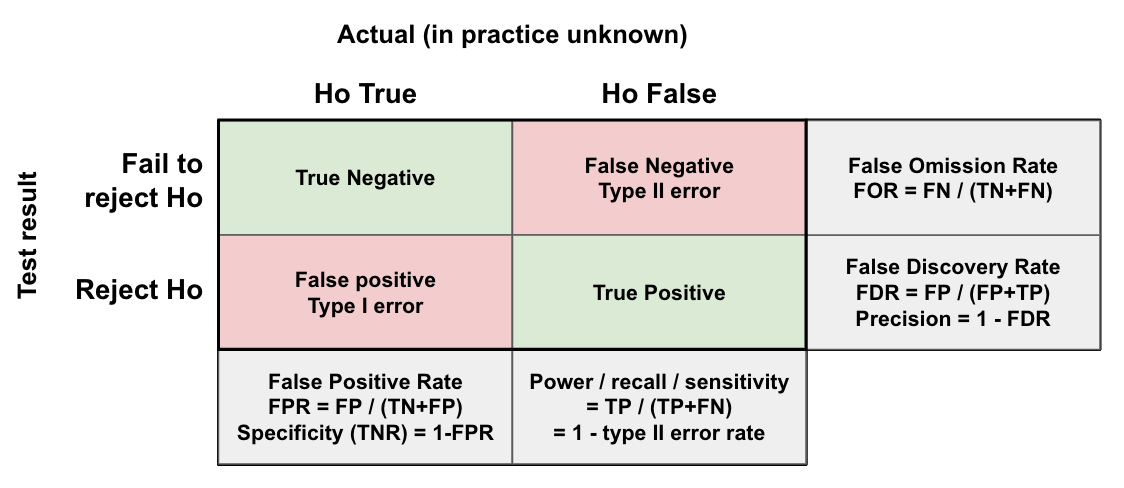
Let’s say only 10% of our 1000 trials are actually effective (100/1000). With 20% power and a 5% significance level we expect 0.2 * 100 = 20 True Positives, and 0.05 * 900 = 45 False Positives. Giving a FDR of 45/(20+45) = 69%. Meaning the majority of our ‘successful’ experiments are actually False Positives. If we increase our power to 80%, we expect 0.8 * 100 = 80 True Positives, giving a FDR of 45/(80+45) = 36%. A notable improvement. This is why we should always aim for a relatively high power (e.g. 80%), to ensure we can trust the results of our experiment.

The problem with post-hoc (observed) power

Importantly, the power analysis should be done before you run your experiment or analysis. Observed or ad-hoc power based on the observed effect and sample size is essentially a re-arrangment of the test formula, so it’s directly related to the p-value and adds no new information. If the p-value is not significant, the post-hoc power will be less than 50% (and vice versa) as shown below (Hoenig & Heisey, 2001). It’s also been demonstrated through simulations that the post-hoc observed power is not informative of the true power (Zhang et al., 2019).

Observed power

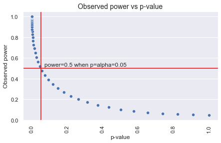
This differs to statistical power (the probability of detecting an effect when one exists), in that statistical power depends on the actual effect size (which is unknown). If a power analysis was not done pre-experiment/analysis for some reason, then you can still do it post to understand the sensitivity of the test (Gelman, 2018). However, the effect size should always be based on what is the minimum meaningful effect for your use case (or a scientifically grounded assumed effect size as mentioned by Gelman in the link above). It should not in any way be related to the observed effect. In the case of experiments, if you don’t have historical data, you could run for a few days first to get the base statistic value and daily number of observations to calculate runtime, but again, the observed effect should not be used.

A similarly flawed version of this is running until you see a significant result, and then calculating the power to decide if you stop the experiment. This has exactly the same problem as above, you’re only re-iterating that the p-value is or isn’t significant.

Formulas: comparing 2 independent random samples

A rule of thumb for the sample size is given by:

\[n = 16 \frac{\sigma^2}{\delta^2}\]

Where \(\delta\) is the minimum detectable effect, and \(\sigma^2\) is the variance. For a binomial metric the variance is:

\[\sigma^2 = p(1-p)\]

Two samples: difference in means

Assuming the means follow normal distributions (i.e. the sampling distribution of the estimator is normal), we can use a normal approximation as shown below (source).

\[k = \frac{n_a}{n_b}\] \[n_b = (1 + \frac{1}{k})(\sigma \frac{z_{1-\alpha} + z_\text{power}}{\mu_\text{difference}})^2\] \[n_a = k * n_b\]

import numpy as np
import scipy.stats as stats

def sample_size_mean_difference(base_mean, base_stddev, mde, mde_type='relative', alternative='two-sided', alpha=0.05, power=0.8, ratio=1):
    """
    Calculates the total sample size required to compare the means of two independent random samples,
    assuming the means follow normal distributions.
    base_mean: The estimated mean for the control group (value pre-experiment).
    base_stddev: The estimated standard deviation for the control group (value pre-experiment).    
    mde: Desired minimum detectable effect
    mde_type: relative (percentage of base e.g. 0.1 for 10% uplift) or absolute (muB-muA)
    alternative: Whether the hypothesis is one ('one-sided') or two sided (default).
    alpha: The significance level (False Positive Rate).
    power: The desired power (chance of detecting an effect when one exists).
    ratio: The ratio of the number of observations in A relative to the total (=nA/nB).
    E.g. for an equal split (50%/50%) it's 1:1 or 1/1, so the ratio=1. 
    For 10% in A and 90% in B, the ratio=1/9. Inversely, for 90% in A, the ratio=9/1.
    Returns: total sample size, sample size for group A and sample size for group B.
    """

    if mde_type == 'relative':
        effect_size = mde * base_mean
    else:
        effect_size = mde
        
    if alternative == 'two-sided':
        alpha_test = alpha/2
    elif alternative == 'one-sided':
        alpha_test = alpha
    else:
        print('Error: unknown alternative')
        return None, None, None

    z_alpha = stats.norm.ppf(1 - alpha_test)
    z_power = stats.norm.ppf(power)
    a = (z_power+z_alpha)**2
    b = (base_stddev / mde)**2
    
    nB = (1 + 1/ratio) * a * b
    nA = (1 + ratio) * a * b
    
    return int(np.ceil(nA)) + int(np.ceil(nB)), int(np.ceil(nA)), int(np.ceil(nB))

Example: testing against statsmodels calculator for t-test

effect = muB - muA
sd=10
std_effect_size = effect / sd
alpha=0.05
beta=0.20
kappa=1

nt, na, nb = sample_size_mean_difference(base_mean=muA,
                                         base_stddev=10, 
                                         mde=effect,
                                         mde_type='absolute',
                                         base_stddev=sd, 
                                         alternative='two-sided', 
                                         alpha=alpha, 
                                         power=1-beta, 
                                         ratio=kappa)

print('Total sample = {} (A={}, B={})'.format(nt, na, nb))

Total sample = 126 (A=63, B=63)

from statsmodels.stats.power import tt_ind_solve_power
nb_sm = tt_ind_solve_power(effect_size=std_effect_size, 
                           alpha=alpha, 
                           power=1-beta, 
                           ratio=kappa, 
                           alternative='two-sided')

print('Number in group B: {:.0f}'.format(nb_sm))

Number in group B: 64

Note, for large samples the normal approximation will be very close to the t-distribution. However, for smaller samples, the t-distribution should be used. This requires simulating different values as the t-distribution depends on the degrees of freedom, which in turn depends on the sample size. For this you can use the statsmodels function above (or similar).

Two samples: difference in proportions

For example, you want to compare the conversion rate in the control and variant groups.

Definitions (source):

\[k=\frac{n_A}{n_B}\] \[n_B = ( \frac{p_A(1-p_A)}{k} + p_B(1-p_B) ) ( \frac{z_{1-\alpha} + z_\text{power}}{p_\text{difference}} )^2\] \[n_A = k * n_B\]

import numpy as np
import scipy.stats as stats

def sample_size_binary(base_rate, mde, mde_type='relative', alternative='two-sided', alpha=0.05, power=0.8, ratio=1):
    """
    Calculates the total sample size required to compare proportions in two independent random samples,
    assuming the normal distribution is a good approximation for the binomial.
    Based on: http://powerandsamplesize.com/Calculators/Compare-2-Proportions/2-Sample-Equality
    base_rate: The proportion in the control group.
    mde: Desired minimum detectable effect
    mde_type: relative (percentage of base e.g. 0.1 for 10% uplift) or absolute (pB-pA)
    alternative: Whether the hypothesis is one ('one-sided') or two sided (default). Changes alpha.
    alpha: The significance level (False Positive Rate).
    power: The desired power (chance of detecting an effect when one exists).
    ratio: The ratio of the number of observations in A relative to the total (=nA/nB).
    E.g. for an equal split (50%/50%) it's 1:1 or 1/1, so the ratio=1. 
    For 10% in A and 90% in B, the ratio=1/9. Inversely, for 90% in A, the ratio=9/1.
    Returns: total sample size, sample size for group A and sample size for group B.
    """
    
    if mde_type == 'relative':
        effect_size = mde * base_rate
    else:
        effect_size = mde
        
    if alternative == 'two-sided':
        alpha_test = alpha/2
        
    elif alternative == 'one-sided':
        alpha_test = alpha
    
    else:
        print('Error: unknown alternative')
        return None, None, None

    variant_rate = base_rate + effect_size
    z_alpha = stats.norm.ppf(1 - alpha_test)
    z_power = stats.norm.ppf(power)
    a = ((z_power+z_alpha) / effect_size)**2
    b = base_rate*(1-base_rate)/ratio + variant_rate*(1-variant_rate)

    nB = a * b
    nA = ratio * nB
    
    return int(np.ceil(nA)) + int(np.ceil(nB)), int(np.ceil(nA)), int(np.ceil(nB))

Example:

pA=0.65
pB=0.85
kappa=1
alpha=0.05
beta=0.20

na, nb, nt = sample_size_binary(base_rate=pA, 
                                mde=pB-pA, 
                                mde_type='absolute', 
                                alternative='two-sided', 
                                alpha=alpha, 
                                power=1-beta, 
                                ratio=kappa)

print('Total sample = {} (A={}, B={})'.format(nt, na, nb))

Total sample = 70 (A=140, B=70)

Checked the results here, and it matches.

Simulating different settings

It’s also useful to plot the sample size required based on different settings for the minimum detectable effect, error rates, and/or ratio (for designs with an unequal split). Ultimately, we have to decide what is a meaningful difference based on our use case, but sometimes we might be willing to trade this off with runtime (e.g. I might not be willing to wait more than 2 weeks, so I’ll accept a higher min. detectable effect).

Runtime vs Minimum Detectable Effect

import numpy as np
import scipy.stats as stats
import seaborn as sns
import matplotlib.pyplot as plt

plt.style.use('ggplot')
sns.set(style='dark')

def runtime_vs_mde(base_statistic, base_std_deviation, observations_per_day, metric_type, relative_effect_list, alternative='two-sided', power=0.8, alpha=0.05, ratio=1, plot=True):
    """
    Calculate required runtime for a variety of effect sizes (minimum detectable effects).
    base_statistic (float): Baseline mean or proportion.
    base_std_deviation (float): Baseline standard deviation (None if binomial).
    observations_per_day (float): Estimated daily traffic (to calculate runtime).
    metric_type (string): 'continuous' or 'binary'.
    relative_effect_list (list(float)): list of relative effects to test (e.g. [x.round(1) for x in np.arange(0.1, 0.6, 0.1)] tests from 5% to 50%).
    alternative (string): 'two_sided' or 'one_sided'.
    power (float): Chance of detecting an effect when one exists (default=0.8).
    alpha (float): Significance level (default=0.05, or 5% false positive rate).
    ratio (float): The ratio of the number of observations in A relative to the total (=nA/nB).
    plot: If True, outputs a plot of the results.
    :return: Pandas DataFrame with total sample size and runtime per relative effect.
    """
    
    relative_effects = []
    sample_sizes = []
    runtimes = []
    
    for rel_effect in relative_effect_list:

        abs_uplift = rel_effect * base_statistic
        relative_effects.append(rel_effect)
        
        if metric_type == 'continuous':

            sample_required = sample_size_mean_difference(base_mean=base_statistic, 
                                                          base_stddev=base_std_deviation, 
                                                          mde=abs_uplift, 
                                                          mde_type='absolute', 
                                                          alternative='two-sided', 
                                                          alpha=alpha, 
                                                          power=power, 
                                                          ratio=ratio)[0]

            runtime_days = np.ceil(sample_required/observations_per_day)
            sample_sizes.append(sample_required)
            runtimes.append(runtime_days)

        elif metric_type == 'binary':

            sample_required = sample_size_binary(base_rate=base_statistic,
                                                 mde=abs_uplift, 
                                                 mde_type='absolute', 
                                                 alternative='two-sided', 
                                                 alpha=alpha, 
                                                 power=power, 
                                                 ratio=ratio)[0]

            runtime_days = np.ceil(sample_required/observations_per_day)
            sample_sizes.append(sample_required)
            runtimes.append(runtime_days)

        else:
            print('Error: unknown metric type')
            sample_sizes.append(None)
            runtimes.append(None)

    estimates_df = pd.DataFrame({'relative_effect': relative_effects,
                                 'total_observations_required': sample_sizes,
                                 'runtime_days': runtimes
                                 })
    
    # Plot
    if plot == True:
        fig, axs = plt.subplots(1, 1, figsize=(7, 4), squeeze=False)
        sns.scatterplot(data=estimates_df, x="runtime_days", y="relative_effect", ax=axs[0,0])
        axs[0,0].yaxis.grid()
        axs[0,0].yaxis.set_major_formatter(mtick.PercentFormatter(1))
        axs[0,0].set_ylim(0,)
        axs[0,0].set_xlabel('Runtime (days)')
        axs[0,0].set_title('Minimum detectable effect (relative to base) vs runtime', fontsize=14)
        plt.setp(axs[0,0].xaxis.get_majorticklabels(), rotation=90)
        plt.show()

    return estimates_df

Example

muB = 10
muA = 5
sd=10
alpha=0.05
beta=0.20
ratio=1

df_mde = runtime_vs_mde(base_statistic=muA, 
                        base_std_deviation=sd, 
                        observations_per_day=1000, 
                        metric_type='continuous', 
                        relative_effect_list=[0.05, 0.1, 0.15, 0.2, 0.25, 0.3], 
                        alternative='two-sided', 
                        power=1-beta, 
                        alpha=alpha, 
                        ratio=ratio,
                        plot=True)

Min effect vs runtime

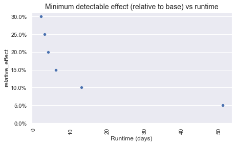
As demonstrated, the runtime increases as the minimum detectable effect decreases.

Runtime vs sampling ratio

import numpy as np
import scipy.stats as stats
import seaborn as sns
import matplotlib.pyplot as plt

plt.style.use('ggplot')
sns.set(style='dark')

def runtime_vs_ratio(base_statistic, base_std_deviation, observations_per_day, metric_type, mde, sampling_ratio_list, alternative='two-sided', power=0.8, alpha=0.05, plot=True):
    """
    Calculate required runtime for a variety of sampling ratios (control/variant splits).
    base_statistic (float): Baseline mean or proportion.
    base_std_deviation (float): Baseline standard deviation (None if binomial).
    observations_per_day (float): Estimated daily traffic (to calculate runtime).
    metric_type (string): 'continuous' or 'binary'.
    mde: Desired minimum detectable effect (% uplift on base_statistic).
    sampling_ratio_list (list(float)): list of ratios to test, where ratio=nA/nB (e.g. [1/9, 2/8, 3/7, 4/6, 5/5, 6/4, 7/3, 8/2, 9/1]).
    alternative (string): 'two_sided' or 'one_sided'.
    power (float): Chance of detecting an effect when one exists (default=0.8).
    alpha (float): Significance level (default=0.05, or 5% false positive rate).
    plot: If True, outputs a plot of the results.
    :return: Pandas DataFrame with total sample size and runtime per sampling ratio.
    """
    
    sampling_ratios = []
    sample_sizes = []
    runtimes = []
    
    for ratio in sampling_ratio_list:

        abs_uplift = mde * base_statistic
        sampling_ratios.append(ratio)
        
        if metric_type == 'continuous':

            sample_required = sample_size_mean_difference(base_mean=base_statistic, 
                                                          base_stddev=base_std_deviation, 
                                                          mde=abs_uplift, 
                                                          mde_type='absolute', 
                                                          alternative='two-sided', 
                                                          alpha=alpha, 
                                                          power=power, 
                                                          ratio=ratio)[0]

            runtime_days = np.ceil(sample_required/observations_per_day)
            sample_sizes.append(sample_required)
            runtimes.append(runtime_days)

        elif metric_type == 'binary':

            sample_required = sample_size_binary(base_rate=base_statistic,
                                                 mde=abs_uplift, 
                                                 mde_type='absolute', 
                                                 alternative='two-sided', 
                                                 alpha=alpha, 
                                                 power=power, 
                                                 ratio=ratio)[0]

            runtime_days = np.ceil(sample_required/observations_per_day)
            sample_sizes.append(sample_required)
            runtimes.append(runtime_days)

        else:
            print('Error: unknown metric type')
            sample_sizes.append(None)
            runtimes.append(None)

    estimates_df = pd.DataFrame({'sample_ratio': sampling_ratios,
                                 'total_observations_required': sample_sizes,
                                 'runtime_days': runtimes
                                 })
    
    # Plot
    if plot == True:
        fig, axs = plt.subplots(1, 1, figsize=(7, 4), squeeze=False)
        sns.scatterplot(data=estimates_df, x="runtime_days", y="sample_ratio", ax=axs[0,0])
        axs[0,0].yaxis.grid()
        axs[0,0].set_ylim(0,)
        axs[0,0].set_xlabel('Runtime (days)')
        axs[0,0].set_title('Sample ratio vs runtime', fontsize=14)
        plt.setp(axs[0,0].xaxis.get_majorticklabels(), rotation=90)
        plt.show()

    return estimates_df

Example:

muB = 10
muA = 5
sd=10
alpha=0.05
beta=0.20

df_mde = runtime_vs_ratio(base_statistic=muA, 
                          base_std_deviation=sd, 
                          observations_per_day=1000, 
                          metric_type='continuous', 
                          mde=0.1,
                          sampling_ratio_list=[1/9, 2/8, 3/7, 4/6, 5/5, 6/4, 7/3, 8/2, 9/1], 
                          alternative='two-sided', 
                          power=1-beta, 
                          alpha=alpha, 
                          plot=True)

Min effect vs runtime

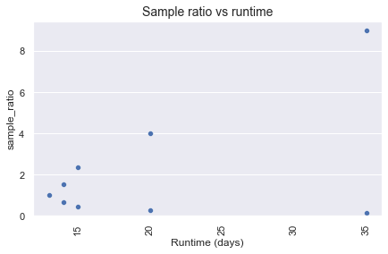
As demonstrated, the runtime increases as the sampling ratio moves away from 1:1.

Creating an experiment plan

A trustworthy experiment should have the following outlined in a plan before the experiment starts:

Objectives of the test (e.g. what is your hypothesis, reasoning, and assumptions);
How the data will be collected (e.g. all visitors who go to page X on web), and the allocation/sampling ratio (e.g. 50%/50% into control and variant);
Primary and supporting metrics, and the expected result for each (e.g. primary metric should increase by more than some defined min. detectable effect);
What statistical tests you will use, and the settings for significance (alpha), and power (1-beta);
Runtime or sample size required based on a power analysis; and,
Decision criteria (e.g. what results would lead you to approve the treatment for all?).

Final Thoughts:

Power is the probability of detecting an effect when one exists. The standard error (variation of the sampling distribution) decreases as the sample increases, improving the power. However, we could also increase the significance level (accept more False Positives), or target larger effects (increase minimum detectable effect), to improve the power.
A low power doesn’t just reduce your chances of detecting real effects, it can also result in most of your ‘positive’ results being False Positives (high False Discovery Rate). Therefore, even if you get a positive result, if the power is low the trustworthiness of the result is questionable. This is why it’s important to control the power with a power analysis pre-experiment.
Post-hoc/observed power analysis is not very useful unless you use the same process as pre-experiment for the effect size (i.e. use the min. meaningful effect). It should not be based on the observed effect as this is then just another way of expressing the p-value (they’re directly linked).
For the t-test, the formula depends on the degrees of freedom (which in turn depends on n), so to calculate the sample size we need to simulate different values. The statsmodels power functions do this for you. They also have some nice plotting functions built in!
For a non-inferiority test, subtract the threshold from the mean difference (more here).
Regardless of the power analysis results, most companies recommend running an experiment for at least a week to capture day of week variation, and in general round up to whole weeks for this same reason.
The power analysis is typically focused on the primary metrics of interest. However, if you want to ensure you also have sufficient power to detect effects in supporting metrics, or different segments, then you can also run the same analysis for these (using the maximum sample size as the final number). However, you may want to correct for multiple testing by lowering the significance level (more strict) for supporting metrics.
Due to the high variance of many continuous metrics (e.g. amount spent is typically skewed), binary metrics like conversion typically require a smaller sample size. However, this shouldn’t be the only reason for using a binary metric as the primary. It first of all should align with your hypothesis.

Other references:

→