Probability refresher
The goal of probability theory is to quantify uncertainty. Once an event occurs, the outcome is known (e.g. it rained today or it didn’t). However, before an event happens, probability allows us to assess the likelihood of various potential outcomes (e.g. the chance that it will rain). Depending on the relationship between events, probability rules help us calculate the likelihood of a given outcome in a straightforward manner. A fundamental concept in probability is that of random variables, which assign numerical values to the outcomes of random processes. These random variables can take different forms: discrete, where the outcomes are countable (such as the number of heads in a series of coin flips), or continuous, where the outcomes can take any value within a given range (such as the height of a person). Understanding and applying probability theory equips us to make informed decisions based on the inherent uncertainty in real-world phenomena. Below I’ll summarise some of the key concepts that are relevant for Data Scientists.
Random Variables
A random variable (also called a stochastic variable) is a function that assigns numerical values to the outcomes of a random event. These outcomes are drawn from a sample space, which is the set of all possible results. For instance, when flipping a fair coin, there are two equally likely outcomes: heads or tails. If we define a random variable X that assigns 1 to heads and 0 to tails, the probabilities for each are: P(H)=P(T)=½, which add to 1. Random variables can be:
- Discrete: Taking values from a finite or countable set, such as the number of heads in a series of coin flips. The probability distribution for discrete random variables is described by a probability mass function (PMF).
- Continuous: Taking values from an uncountable range, such as the height of a person, which can vary continuously. For continuous variables, the probability distribution is described by a probability density function (PDF).
- Mixture: Sometimes random variables have a combination of discrete and continuous components (e.g. blood results where below a threshold it’s “undetectable” (0 has some probability), but above that it’s a continuous value, meaning no specific value has a positive probability).
In statistics, random variables are usually considered to take real number values, which allows us to define important quantities like the expected value (mean), and variance.
Distributions
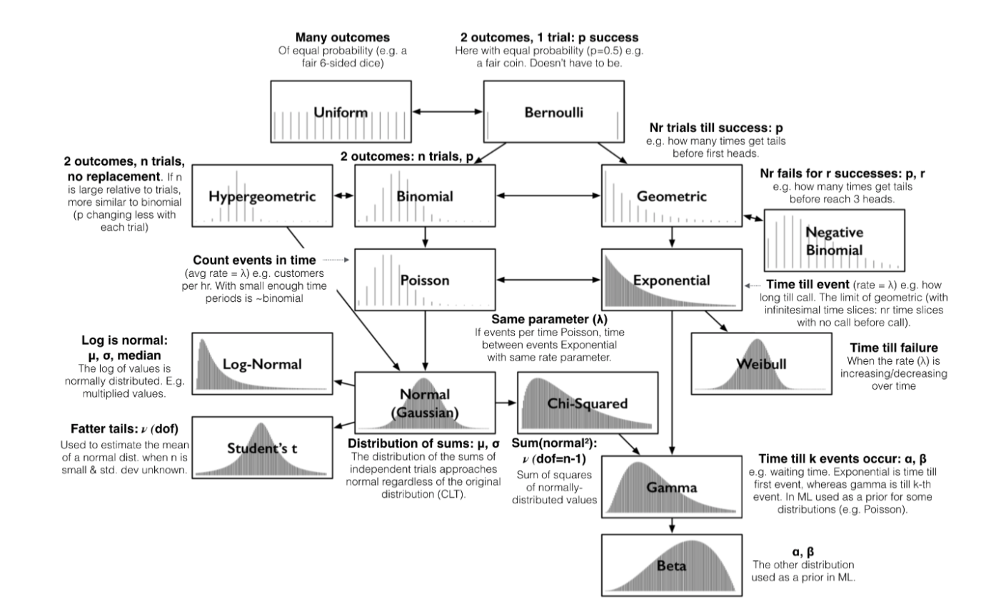
A probability distribution lists all possible outcomes of a random variable along with their corresponding probabilities (must sum to 1). Rather than listing all possible probabilities, we can define a function f(x) that gives the likelihood of certain outcomes in a random process. Some of the most common probability distributions are shown below:
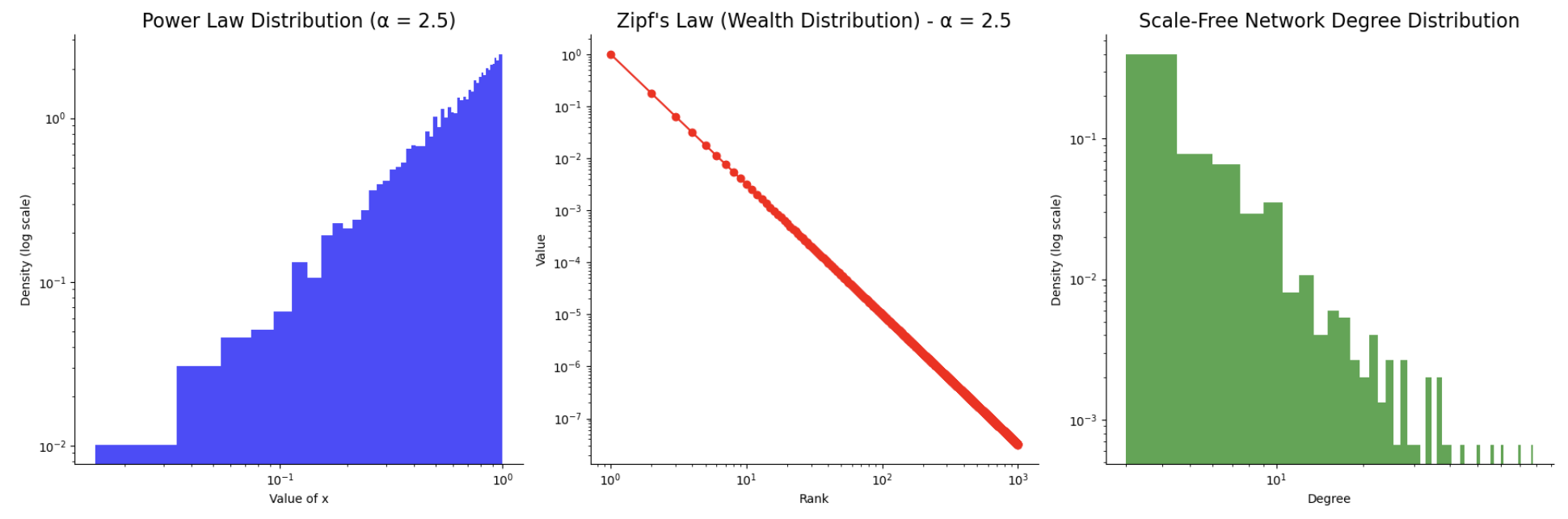
Another one that comes up is the power law distribution: one quantity varies as a power of another (\(y=x^\text{\alpha}\), where y is the dependent, x is the independent and \(\alpha\) is a constant). It has heavy tails (few large values dominate, while many smaller values are common) and scale invariance (the system behaves similarly at different scales, so the pattern remains consistent even when zooming in or out). The extreme values or outliers (like the largest city or the richest person) have a disproportionate effect compared to the “average” values, making it important to understand and account for these distributions in analysis and modelling. Some examples:
- Zipf’s law is a specific type of power law that describes how wealth, population, or even word frequency is distributed. In Zipf’s law, the rank r of an item is inversely proportional to its frequency f, meaning the most frequent item is far more common than the next most frequent, and so on. E.g. the largest city might have 10 million people, the second-largest 5 million, the third-largest 2 million, and so on. The number of cities with these population sizes follows a power law distribution.
- Scale-free networks are characterized by a small number of highly connected nodes (hubs) and many nodes with fewer connections. These networks follow a power law distribution in terms of their degree (the number of connections each node has). Most nodes have few connections, but a few nodes have disproportionately large numbers of connections. Examples include social networks (where a few individuals have many followers) or the internet (where a few websites receive the majority of traffic).
When plotted, it typically produces a curve that starts high and quickly tapers off, which can make it difficult to directly see the relationship. However, if we plot the logarithm of both the variable and the frequency, the relationship becomes linear:
The few extreme events can dominate the mean and even the variance. These aren’t outliers but expected features of a power law distribution (e.g. the largest customer, city, or influencer will be orders of magnitude larger than the average). In practice, examine distributions on a log-log scale to identify them, report medians or percentiles rather than means, and stress-test systems against extreme cases. Useful methods include nonparametric tests such as the Mann-Whitney U for testing, bootstrapped confidence intervals and quantile regression for estimation, and tail-aware models like Pareto or log-normal fits, robust regression, or simulations focused on top contributors for modelling.
PMF / PDF / CDF
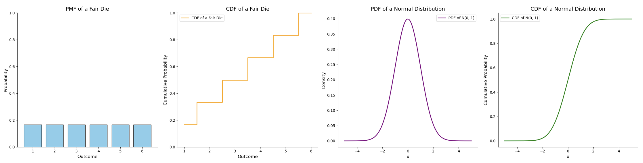
The distributions shown above can be categorised as either a Probability Mass Function (PMF) or Probability Density Function (PDF) depending on the outcome type:
| Metric | Formula | Description |
|---|---|---|
| Probability Mass Function (PMF) | \(P(X = x)\) | Describes the probability distribution of a discrete random variable. The PMF gives the probability that a discrete random variable is exactly equal to some value. For example, in a coin toss, the probability of heads or tails. |
| Probability Density Function (PDF) | \(f(x) = \frac{d}{dx} P(X \leq x)\) | Describes the probability distribution of a continuous random variable. The PDF defines the probability of the random variable falling within a particular range of values, and its integral over an interval gives the probability. The total area under the curve equals 1. |
| Cumulative Distribution Function (CDF) | \(F(x) = P(X \leq x) = \int_{-\infty}^{x} f(t) dt\) | Gives the probability that a random variable is less than or equal to a certain value. For a discrete variable, it’s the sum of the probabilities of all outcomes less than or equal to (x). For a continuous variable, it’s the area under the PDF curve up to (x). |
Moments
Moments are used to describe the shape of the distribution. Each “moment” provides different information about the distribution’s characteristics. Here’s the first few moments:
- Zeroth moment: The total probability, which is always 1.
- First moment: The expected value (mean), which gives the central location of the distribution.
- Second central moment: The variance, which measures the spread of the data around the mean.
- Third standardized moment: The skewness, which describes the asymmetry of the distribution.
- Fourth standardized moment: The kurtosis, which measures the “tailedness” or how extreme the values in the distribution are.
Expected Value
The expected value represents the average outcome over the long run. We calculate it by multiplying each numerical outcome by its probability and summing these products. Consider a game where there is a 4/10 chance of winning $2, a 4/10 chance of losing $5, and a 2/10 chance of winning $10. The expected value is:
\[\frac{4}{10} \cdot 2 + \frac{4}{10} \cdot (-5) + \frac{2}{10} \cdot 10 = 0.8 - 2 + 2 = 0.8\]On average, we expect to win 80 cents per game in the long run. In statistics, this concept is analogous to the population mean, which is often estimated from the sampling distribution, the probability distribution of outcomes obtained from many samples.
Linearity of Expectation
The expected value has a useful property called linearity, which holds even if variables are dependent. The expected value of a sum equals the sum of the expected values:
\[E[X + Y] = E[X] + E[Y]\]This property extends to any finite sum of random variables:
\[E\Big[\sum_{i=1}^n X_i\Big] = \sum_{i=1}^n E[X_i]\]Linearity of expectation makes it easy to compute averages and total outcomes in complex systems without needing to know the dependence structure between variables.
Example: Suppose we roll two dice, $X_1$ and $X_2$, and want the expected sum. Each die has an expected value of 3.5. Even if the dice were somehow dependent, the expected sum is still:
\[E[X_1 + X_2] = E[X_1] + E[X_2] = 3.5 + 3.5 = 7\]Variance
Variance measures how much the outcomes of a random variable spread around the expected value. For a discrete random variable X with outcomes $x_i$ and probabilities $p_i$, the variance is defined as:
\[\text{Var}(X) = E[(X - E[X])^2] = \sum_i p_i (x_i - E[X])^2\]In the earlier game example, variance tells us how much each game’s outcome deviates from the expected value of 0.8. Higher variance indicates more spread in the outcomes, corresponding to greater risk or uncertainty.
Variance Decomposition
Unlike the expected value, variability depends on how values deviate from their mean, so it is not generally additive across dependent variables. Meaning we can’t simply sum the variances of two variables unless they are independent. Instead, we can break down the variability of $X$ with respect to another variable $Y$ using the law of total variance:
\[\text{Var}(X) = E[\text{Var}(X \mid Y)] + \text{Var}(E[X \mid Y])\]Here, $E[\text{Var}(X \mid Y)]$ represents the average variability within groups defined by Y, and $\text{Var}(E[X \mid Y])$ represents the variability of the group means themselves.
Example: Consider test scores for two classes.
- Class A: 3 students scored 70, 75, 80 → mean = 75, variance = 25
- Class B: 3 students scored 80, 85, 90 → mean = 85, variance = 25
If we combine all 6 students:
- Within-class variance (average of the class variances) = (25 + 25)/2 = 25
- Between-class variance (variance of the class means 75 and 85) = 50
- Total variance = within-class + between-class = 25 + 50 = 75
The total variability comes both from differences within each class and differences between class averages, showing why variance requires careful treatment compared with expectation.
Set notation
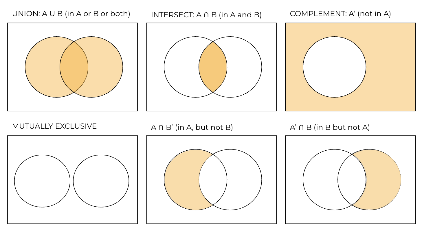
A set is simply a collection of distinct elements. In probability, we often deal with sets to define events and sample spaces. The sample space (denoted as S) is the set of all possible outcomes (e.g. S={H, T}). An event is any subset of the sample space (e.g. the event that the coin lands on heads can be represented as A={H}). When describing relationships between events, we use set notation:
Marginal (unconditional) probability
This is just the probability of A (P(A)).
Complement rule
The probability that something doesn’t happen is 1 minus the probability that it does happen: \(P(A^c)= 1-P(A)\). The probability of something not happening is often easier to compute, so we can take advantage of that.
Example: Assuming the days are independent, what is the probability of at least 1 day of rain in the next 5 days if the P(rain)=0.2 each day?
- The complement of “at least one day of rain” is “no rain at all” over the 5 days.
- Since the days are independent, the probability of no rain on a given day is 1−P(rain)=1−0.2=0.8. For 5 independent days with no rain, the probability of no rain on all 5 days is simply the product of the probabilities for each day: \(P(no rain)= 0.8^5\).
- Therefore, the probability of at least one day of rain is \(P(rain)= 1 - 0.8^5\).
- This is much simpler than directly computing it: summing the probability of rain on exactly 1 day, exactly 2 days, and so on, up to 5 days, then accounting for overlaps and intersections (the joint probabilities).
Conditional Probability
The probability of event A occurring, given that event B has already occurred. The formula for conditional probability is:
\[P(A \mid B) = \frac{P(A \cap B)}{P(B)}\]Divide joint probability of A and B, by the marginal probability of B.
Impact of dependence
Independent events are events where the occurrence of one event does not affect the occurrence of another. For example, in two independent coin flips, the outcome of the first flip does not affect the outcome of the second flip.
- Addition rule (A or B): If mutually exclusive (can’t happen at the same time) then \(P(A \cup B) = P(A) + P(B)\), if they’re not mutually exclusive (e.g. getting H on a coin and rolling a 4): \(P(A \cup B) = P(A) + P(B) - P(A \cap B)\). The P(A∩B) is subtracted once to avoid double counting it in A and B.
- Multiplication rule (A and B): \(P(A \cap B) = P(A) \times P(B)\)
Dependent events are events where the occurrence of one event affects the probability of the other event. An example of this is drawing cards without replacement from a deck. If you draw a card and don’t replace it, the probability of drawing another specific card changes.
- Multiplication rule (A and B): \(P(A \cap B) = P(A) \times P(B \mid A)\)
Odds
Odds are a different way of expressing the likelihood of an event. While probability is the ratio of favorable outcomes to total outcomes, odds are typically expressed as the ratio of favorable outcomes to unfavorable outcomes. For example, if you have a 1 in 5 chance of winning, the odds are 1:4. Odds magnify probabilities, so they allow us to compare probabilities more easily by focusing on large whole numbers. For example, comparing probabilities 0.01 and 0.005 is difficult to interpret directly, but the odds 99:1 vs 199:1 make it easier to see that one is roughly twice as likely as the other.
The table below shows how probabilities map to odds. Notice that when the probability is 0.5 (a 50/50 chance), the odds are 1:1 (“even odds”). This is the natural dividing line: probabilities above 0.5 correspond to odds greater than 1:1, while probabilities below 0.5 correspond to odds less than 1:1.
| Probability (p = odds / (1 + odds)) | Odds (odds = p / (1-p)) | Probability spoken as “1 in …” |
|---|---|---|
| 0.01 | 1:99 | 1 in 100 |
| 0.05 | 1:19 | 1 in 20 |
| 0.10 | 1:9 | 1 in 10 |
| 0.20 | 1:4 | 1 in 5 |
| 0.25 | 1:3 | 1 in 4 |
| 0.33 | 1:2 | 1 in 3 |
| 0.50 | 1:1 | 1 in 2 (“even odds”) |
| 0.75 | 3:1 | 3 in 4 |
| 0.90 | 9:1 | 9 in 10 |
| 0.95 | 19:1 | 19 in 20 |
| 0.99 | 99:1 | 99 in 100 |
Application
Most Data Scientists are familiar with odds from logistic regression, which models a binary outcome by taking the log of the odds (log-odds) of the event, mapping probabilities from the range [0,1] onto the continuous scale (-∞, ∞). Below the tipping point of $p = 0.5$, the log-odds become negative, reflecting that the event is more likely not to occur than to occur. The resulting coefficients describe how a one-unit change in a feature affects the log-odds of the outcome. Exponentiating the coefficients gives the odds ratio, which tells us how the odds of the event change for a one-unit increase in the feature.
For example, suppose we are predicting lung cancer, and the coefficient for smoking is β = log(2) ≈ 0.693. The odds ratio is e^β = 2, meaning smokers have twice the odds of developing the illness compared to non-smokers. The odds ratio compares the odds of two groups, so in this example the odds could be 1:4 for non-smokers and 1:2 for smokers, giving the odds ratio of 0.5 / 0.25 = 2.
For individual level predictions, probabilities are usually more intuitive, so the predicted log odds for each observation is typically converted to a probability:
\[p_i = \frac{e^{\text{log-odds}_i}}{1 + e^{\text{log-odds}_i}}\]| Observation | Feature | Log-odds | Odds | Probability |
|---|---|---|---|---|
| 1 | Smoking = 1 | 0.693 | 2:1 | 0.667 |
| 2 | Smoking = 0 | -0.693 | 1:2 | 0.333 |
A threshold can then be applied to decide the predicted class (e.g. p > 0.5 = 1, else 0), with the cutoff tuned to balance recall (also called sensitivity or true positive rate: % of positive class correctly predicted), and precision (% of predicted positives that are actually positive).
Combinations and permutations
Combinations and permutations are used to count the number of ways outcomes can be arranged:
- Combinations count the number of ways to select a subset of objects where the order does not matter. We write nCk (n choose k) to represent the number of ways to form a combination of k items from n items. 100C100=1 as it’s the same as selecting all.
- Permutations count the number of ways to arrange a set of objects where the order matters. We can write nPk, which the ways we can form k items from n items, counting different orderings of the same set. This will be greater than or equal to nCk.
Bayes’ Theorem
Bayes’ Theorem is the consequence of rearranging the conditional probability formula:
\[P(A \mid B) = \frac{P(B \mid A)P(A)}{P(B)}\]Where:
- \(P(A \mid B)\) is the posterior probability (what we want to find),
- \(P(B \mid A)\) is the likelihood (how likely we are to observe the evidence if the hypothesis is true),
- P(A) is the prior probability (our initial belief),
- P(B) is the marginal likelihood (the total probability of the evidence).
It can also be written as: posterior = likelihood * prior / evidence.
Example: A box contains 8 fair coins (heads and tails) and 1 coin which has heads on both sides. I select a coin randomly and flip it 4 times, getting all heads. If I flip this coin again, what is the probability it will be heads?
- Fair coin: \(P(H \mid fair)=0.5\)
- Biased coin: \(P(H \mid not fair)=1\)
- Prior probability of selecting a fair coin: P(fair) = 8/9
- Conditional probability of 4 H given it’s a fair coin: \(P(4 heads \mid fair) = 0.5^4 = 0.0625\)
- Conditional probability of 4 H given it’s an unfair coin: \(P(4 heads \mid not fair) = 1\)
- Total probability of 4 H: P(4 heads) = 8/90.0625 + 1/91
- Now, use Bayes’ Theorem to calculate the probability that the coin is fair, given that we observed 4 heads: \(P(fair \mid 4 heads) = P(4 heads \mid fair)*P(fair) / P(4 heads) = 0.0625 * 8/9 / 8/9*0.0625 + 1/9*1 = 1/3\)
- Using this we can calculate the probability that the next flip will be heads: \(P(H) again = 1/3 * P(H \mid F) + 2/3 * P(H \mid not fair) = 1/3 * 1/2 + 2/3 * 1 = 5/6\)
Bayes’ Theorem gives us a principled way to update our beliefs when new evidence arrives, connecting prior knowledge with observed evidence. In other words, it allows us to start with an initial estimate or hypothesis (the prior) and systematically revise it as we gather more data, producing a refined probability (the posterior) that reflects both what we already knew and what we have observed. This is especially useful in situations where uncertainty is inherent, such as diagnosing a disease based on test results. For example, even if a test for a rare disease is highly accurate, the probability that a patient actually has the disease can remain low if the prior probability is very small.
Simpson’s paradox
Simpson’s paradox is a counterintuitive phenomenon that occurs when trends observed in different groups of data reverse when the data is combined. Meaning the aggregated data may lead to a different conclusion. This is a specific type of confounding, where the confounding variable might be the group size or way the data is aggregated across different groups.
Example: Consider two doctors performing two types of surgeries. Doctor A has a higher success rate than Doctor B for both types of surgery individually, but performs the more difficult surgery more often (which has a lower succes rate for both doctors), resulting in a lower overall success rate:
- Doctor A has a 95% success rate for surgery type 1 (easier surgery) and a 50% success rate for surgery type 2 (more difficult surgery).
- Doctor A performs surgery type 1 20% of the time and surgery type 2 80% of the time, so they’re success rate is: (0.2×0.95)+(0.8×0.5)=0.19+0.4=0.59 or 59%.
- Doctor B has a 90% success rate for surgery type 1 and a 10% success rate for surgery type 2.
- Doctor B performs surgery type 1 80% of the time and surgery type 2 20% of the time, so they’re success rate is: (0.8×0.9)+(0.2×0.1)=0.72+0.02=0.74 or 74%.
This is why it’s often useful to break down data into meaningful sub groups to get a more accurate understanding of relationships. We need to consider both the whole and the parts to get the full story.
The Law of Large Numbers and Central Limit Theorem
The Law of Large Numbers (LLN) describes how the average of repeated independent observations converges to the expected value as the number of observations increases, with the speed of convergence depending on the expected value and variance of the underlying distribution. In simple terms: the more data you collect, the more the “average outcome” behaves like what you would expect in theory. Small samples can fluctuate, but larger samples produce averages that closely reflect the true expected value.
Example: Suppose we flip a fair coin multiple times and record the proportion of heads. As the number of flips increases, the sample mean gets closer to the true probability of heads, which is 0.5:
- After 5 flips, we might observe 3 heads → sample mean = 3/5 = 0.6
- After 50 flips, we might observe 26 heads → sample mean = 26/50 = 0.52
- After 500 flips, we might observe 248 heads → sample mean = 248/500 = 0.496
This underpins many statistical practices because it justifies the idea that with enough data, averages become stable and predictable.
Central Limit Theorem (CLT) builds on this idea by describing the distribution of those averages. It states that, the distribution of sample means approaches normality for large, independent, identically distributed (i.i.d.) observations with finite variance, regardless of the original distribution of the data. This is why standard confidence intervals and hypothesis tests can be used even when the underlying data is not normally distributed. However, if the underlying data has heavy tails or infinite variance (like some power law distributions), the convergence may be slower, and normal approximations can be misleading.
Example: Imagine we flip a fair coin 10 times and calculate the proportion of heads. If we repeat this experiment 1,000 times and plot a histogram of the 1,000 sample means, we will see a bell-shaped curve centred around 0.5. Each histogram bar represents the proportion of heads in a 10-flip sample. Even though individual flips are binary, the distribution of the averages across many samples is approximately normal, illustrating the Central Limit Theorem.
The LLN ensures that averages stabilise as we collect more data, while the CLT shows that the distribution of those averages becomes predictable and bell-shaped, allowing us to make reliable inferences from random, variable observations.
Conclusion
Probability allows us to handle uncertainty by quantifying the likelihood of different outcomes. In statistics, it underpins the process of making inferences, testing hypotheses, and predicting future events. For hands-on practice, I would recommend using something like brilliant.org as they have plenty of examples to work through.