Causal inference
The primary goal of this guide is to store my notes, but I hope it may also serve as a practical resource for other data scientists in industry. It begins with an intuitive overview of causal effects and the notation commonly used to describe them, then moves through how to define a causal question, assess identifiability, and estimate effects from data using models. While the framework is grounded primarily in potential outcomes, I also make use of causal diagrams (DAGs) to support the discussion on identification.
If you’d like to skip ahead, here are links to some of the key sections:
- Introduction
- Notation
- Causal treatment effects
- Formulating a causal question (estimands and effect measures)
- Identification in randomised experiments
- Identification in observational studies
- Estimating causal effects with models
- ATE models
- CATE models
- Longitudinal challenges and methods
- Other common methods
- Appendix
- References
Introduction
You have likely heard the phrase “correlation is not causation.” Formally, we would say a treatment has a causal effect on an individual if their outcome under treatment differs from what it would have been without it. This includes both active interventions (like sending an email), and passive exposures (like a policy change or app outage). The fundamental problem is that we can never observe both outcomes for the same individual. If you send a customer an email, you can observe whether they return afterward, but you will never know for sure what they would have done without it. The potential outcomes framework makes this explicit by distinguishing between the factual (observed outcome) and the counterfactual (unobserved alternative). While we can’t observe both for one individual, we can estimate the average treatment effect (ATE) across groups, provided the treated and untreated are otherwise comparable. Further, by conditioning on relevant variables, we can estimate the conditional average treatment effect (CATE), enabling more personalised decisions.
In randomised experiments, comparability is achieved by design. By randomly assigning treatment, we ensure that differences in outcomes between treated and untreated groups can be attributed to the treatment. However, experiments are not always feasible due to legal, ethical, financial, or logistical constraints. In such cases, we rely on observational data, and distinguishing causation from correlation becomes more difficult. When two variables are associated, observing the value of one, tells us something about the value of the other. However, observing two variables X and Y moving together cannot tell us whether X causes Y, Y causes X, or whether both are caused by a third variable Z. To use a classic example, beer and ice cream sales may rise together in summer, not because one causes the other, but because both are driven by temperature.
Causal inference from observational data requires careful thinking about the data-generating process: defining an intervention (treatment), understanding how treatment is assigned, and clarifying assumptions. For any method to identify causal effects, three core conditions must hold: a well-defined intervention (something concrete needs to be changing), exchangeability (treated and untreated groups are comparable in the absence of treatment), and positivity (every individual has a nonzero probability of receiving each treatment level).
Ultimately, causal claims from observational data rely heavily on domain knowledge and the plausibility of the assumptions. Since perfect data is rare, transparency and sensitivity analyses are essential for assessing potential biases. This transparency is both a strength and a vulnerability, as it invites scrutiny. However, relying on methods with hidden or unacknowledged assumptions does not lead to more trustworthy decisions; it only conceals the uncertainty rather than addressing it.
Description, Prediction, or Explanation?
Before jumping into causal inference theory and methods, it’s crucial to understand where causal questions fit within the broader data science landscape. As a data scientist, you’re often handed vague requests. A critical part of the job is to clarify what the stakeholder is really asking, and what they intend to do with the answer. Most questions fall into one of three broad categories:
-
Descriptive: What is happening? E.g. Where are our users located? What is our market share by region?
Descriptive analysis summarises data to understand current or past conditions, reporting observed patterns without implying causality. The key validity issues are: measurement error (variables recorded inaccurately), and sampling error (the data does not represent the intended population, e.g. survey results can suffer from selection bias).
-
Predictive: What is likely to happen? E.g. Who will churn next month? Which users are likely to convert?
Predictive models use historical patterns to forecast unknown or future outcomes. Their goal is predictive accuracy, evaluated on new data. Variables are chosen based on their ability to improve prediction, regardless of whether they cause the outcome. Predictive models can be used to help rank or segment, but do not tell you which actions will change outcomes. The main validity issues are overfitting and target leakage (resulting in poor out of sample performance).
-
Explanatory (i.e. causal inference): Why did something happen? What would happen if we changed something? E.g. What drives conversion? Would offering a 5 percent discount increase trial conversion rates?
Causal analysis estimates the effect of an intervention or treatment on an outcome, answering what-if questions to guide decision-making. It requires assumptions about the data-generating process, often informed by domain knowledge. The central validity concern is internal validity: whether the estimated effect is credible for the studied group. Though external validity also matters when generalising findings beyond the sample. Unlike predictive models, causal models may not predict outcomes well but provide unbiased estimates of treatment effects when assumptions hold.
Confusion often arises in real-world projects when questions span multiple categories. You might start with descriptive analysis to identify patterns and understand your population, build predictive models to forecast outcomes, and ultimately tackle causal questions about how to influence results. The common mistake is treating these categories as interchangeable. Even when using the same tools, the assumptions, goals, and interpretations differ. Crucially, a model with high predictive accuracy does not necessarily reveal the true effect of any variable. Conversely, a model designed for causal estimation may not excel at prediction. These are fundamentally different tasks.
To illustrate this point, suppose you build a model to predict beer sales, and find that ice cream sales are a strong predictor. The model performs well and the coefficient is significantly positive, so you conclude that increasing ice cream sales will also increase beer sales. However, the true driver is likely weather. Acting on this mistaken belief could waste time, or even reduce overall sales if the two products compete. It is easy to make this mistake. Predictive models often produce convincing results that seem to explain outcomes. When stakeholders want actionable insights, there is pressure to move quickly and skip formal causal analysis. As a result, we often get what Haber et al. (2022) calls “Schrödinger’s causal inference”: an analysis that avoids stating a causal goal, but still makes causal claims and recommendations.
While it often requires more upfront effort, more formal causal thinking prevents teams from pursuing strategies that have no real effect, saving time in the long run by avoiding costly detours.
Choosing the Right Level of Evidence
Causal thinking promotes a deeper understanding of problems by focusing on mechanisms and clarifying assumptions. However, not every causal question requires a full formal study. In many operational settings, a strong correlation paired with contextual knowledge is enough to justify quick action. For example, if conversions drop suddenly and you notice a product change was deployed at the same time, it’s reasonable to suspect the change as the cause and test a rollback. In these cases, you are still reasoning causally, but the cost of being wrong is low, and the response is reversible. The key is to be honest about the level of uncertainty and the type of evidence being used. As a counter example, suppose you’re evaluating whether the company should expand to a new market. Let’s say prior expansions were successful, but focused on high-growth regions. Naively comparing this market to the prior examples may overestimate the expected outcome. The decision is high cost and difficult to reverse, so it would be beneficial to use a more formal causal approach to control for the market differences.
Workflow
The distinction between prediction and causation naturally leads us to the workflow for explanatory questions. If you’ve done a lot of predictive modeling, this will feel familiar, but with some important shifts in mindset. In causal inference, our goal isn’t just to model outcomes well, but to estimate what would happen under different interventions. That means clearly defining counterfactual scenarios and ensuring that our models reflect the underlying data-generating process, rather than aiming for high predictive accuracy.
The workflow below outlines one principled approach to identifying causal effects, though it’s not the only path:
-
1. Specify a causal question: Start by clearly articulating your causal question in terms of an intervention and outcome. For example: What is the effect of weekly promotional emails on time to unsubscribe? This step includes defining the estimand (e.g. average treatment effect on survival at 12 weeks), population, and time horizon.
-
2. Draw assumptions using a causal diagram: Use a diagram (e.g. DAG) to encode your assumptions about the relationships among treatment, outcome, covariates, and possible sources of confounding or bias. This helps identify which variables must be adjusted for to estimate the causal effect.
-
3. Model assumptions: Choose a method that aligns with your causal goal and the structure of your data. Crucially, your model should reflect the causal structure from the DAG, not just predictive performance.
-
4. Diagnostics: Once fit, evaluate how well the models reflect your assumptions. This could involve checking covariate balance after weighting, evaluating model fit and positivity violations, or plotting predicted survival curves under different interventions. Unlike pure prediction, model diagnostics in causal inference focus on plausibility and identifiability, not predictive accuracy metrics.
-
5. Estimate the causal effect: With a well-specified and diagnosed model, compute your causal estimand. This may involve simulation of counterfactual outcomes, and bootstrapping confidence intervals.
-
6. Conduct sensitivity analysis: All causal estimates rest on untestable assumptions (e.g., no unmeasured confounding). Sensitivity analyses help quantify how robust your conclusions are to violations of those assumptions. This might include bounding approaches, bias formulas, or varying model specifications.
I’m presenting this workflow upfront to provide a clear framework for how the pieces fit together. In the next sections, we’ll dive into the theory and notation behind each step, but having the full picture in mind will help keep the details grounded.
Notation
Before we go further, let’s cover some notation and definitions. This will make it easier to follow the explanations, but you can refer back as you go. Note, capital letters are used for random variables, and lower case for particular values of variables.
| Notation / Term | Definition |
|---|---|
| \(T_i\) | Treatment indicator for observation \(i\). Takes the value 1 if treated, 0 if not treated. |
| \(Y_i\) | The observed outcome for observation \(i\). |
| \(Y_{\text{0i}}\) | The potential outcome for observation \(i\) without treatment (i.e., counterfactual under control). |
| \(Y_{\text{1i}}\) | The potential outcome for observation \(i\) with treatment (i.e., counterfactual under treatment). |
| \(Y_{\text{1i}} - Y_{\text{0i}}\) | The individual treatment effect for observation \(i\). This is not directly observable. |
| \(ATE = E[Y_{\text{1}} - Y_{\text{0}}]\) | The average treatment effect (ATE): the expected treatment effect across the entire population. |
| \(ATT = E[Y_{\text{1}} - Y_{\text{0}} \mid T=1]\) | The average treatment effect on the treated (ATT): the expected effect for those who actually received treatment. |
| \(\tau(x) = E[Y_{\text{1}} - Y_{\text{0}} \mid X = x]\) | The conditional average treatment effect (CATE): the expected effect for individuals with covariates \(X = x\). |
| \(\perp\!\!\!\perp\) | Denotes independence. For example, \(A \perp\!\!\!\perp B\) means that variables \(A\) and \(B\) are statistically independent. |
If \(T_i = t\), then \(Y_\text{ti}=Y_i\). That is, if observation i was actually treated (t=1), their potential outcome under treatment equals their observed outcome. Meanwhile, \(Y_t\) denotes the random variable representing the potential outcome under treatment t across the entire population.
An introduction to causal treatment effects
Individual effect
A treatment has a causal effect on an individual’s outcome if their outcome with the treatment differs to their outcome without it. Let’s pretend we have two identical planets, and the only difference is that on Earth 1 no one plays tennis (\(Y^\text{t=0}\)) and on Earth 2 everyone plays tennis (\(Y^\text{t=1}\)). The outcome is whether you get cancer, and the treatment is playing tennis. The table below shows there is a causal effect of tennis on cancer for Alice, Bob and Eva because the difference in the potential outcomes is non-zero. Alice and Eva get cancer if they don’t play tennis, and don’t get cancer if they do. The inverse is true for Bob.
| Name | \(Y^\text{t=0}\) | \(Y^\text{t=1}\) | Difference |
|---|---|---|---|
| Alice | 1 | 0 | -1 |
| Bob | 0 | 1 | 1 |
| Charlie | 1 | 1 | 0 |
| David | 0 | 0 | 0 |
| Eva | 1 | 0 | -1 |
| Fred | 0 | 0 | 0 |
| Average | 3/6 | 2/6 | -1/6 |
Average effect
If we take the average treatment effect in the example above (\(ATE=-\frac{1}{6}\)), we would conclude tennis decreases the chance of you getting cancer. We can also see this in the average cancer rate for those with and without treatment (as the average of the differences is equal to the difference of the averages). With tennis (\(Y^\text{t=1}\)) they had a \(\frac{2}{6}\) chance, whereas without it (\(Y^\text{t=0}\)) they would have had a \(\frac{3}{6}\) chance (\(E[Y^\text{t}] \neq E[Y^\text{t'}]\)). Keep in mind there can be individual causal effects even if there is no average causal effect. For example, Alice has an individual causal effect because she avoids cancer if she plays tennis, even if the average showed no difference. While the average causal effect is most commonly used, you can also use other differences such as the median or variance.
The fundamental problem
The fundamental problem of causal inference is that we can never observe the same person/observation with and without treatment at the same point in time. While we might not be able to measure individual effects, we can measure average effects. This is where potential outcomes comes in: the actual observed outcome is factual and the unobserved outcome is the couterfactual. If we compare those with and without treatment and they are otherwise similar, we can estimate the average effect.
| Name | \(Y^\text{t=0}\) | \(Y^\text{t=1}\) |
|---|---|---|
| Alice | 1 | ? |
| Bob | ? | 1 |
| Charlie | 1 | ? |
| David | ? | 0 |
| Eva | ? | 0 |
| Fred | 0 | ? |
| Average | 2/3 | 1/3 |
Now in our two Earth’s example, if we randomly selected the samples, this would be an unbiased estimate of the average causal effect. However, if we just took a sample of people from our one Earth and compared those who played tennis to those who don’t, we run into the problem of bias because all else is not equal (there are other factors influencing the cancer rate that also impact the likelihood of playing tennis, i.e. confounders). We can say from this there’s an association, but not necessarily causation.
Bias in observational data
Bias is the key concept that separates association from causation. Intuitively, when we compare observational data, we will consider why a difference might exist that isn’t due to the treatment itself. For instance, playing tennis requires time and money, which means tennis players may also have higher incomes and engage in other health-promoting behaviors, such as eating healthy food, and having regular doctor visits. This could explain some or all of the observed difference in cancer rates.
We cannot observe the counterfactual outcome, \(Y_0\), for the tennis group. In other words, we can’t know what their cancer risk would be if they didn’t play tennis. However, we can reason that \(Y_0 \mid T=1\) (the cancer risk of tennis players if they didn’t play tennis) is likely lower than \(Y_0 \mid T=0\) (the cancer risk of non-tennis players), implying that the baseline differs (it’s not a fair comparison). Using the potential outcomes framework we can express this mathematically. An association is measured as the difference in observed outcomes:
\[E[Y \mid T=1] - E[Y \mid T=0] = E[Y_1 \mid T=1] - E[Y_0 \mid T=0]\]We can separate the treatment effect (ATT) and the bias components by first adding and subtracting the counterfactual outcome \(E[Y_0 \mid T=1]\) (the outcome for treated individuals had they not received the treatment):
\[E[Y \mid T=1] - E[Y \mid T=0] = E[Y_1 \mid T=1] - E[Y_0 \mid T=0] + E[Y_0 \mid T=1] - E[Y_0 \mid T=1]\]Then re-arranging the equation:
\[= E[Y_1 - Y_0 \mid T=1] + E[Y_0 \mid T=1] - E[Y_0 \mid T=0]\]Where:
- \(E[Y_1 - Y_0 \mid T=1]\) represents the Average Treatment Effect on the Treated (ATT), i.e. the treatment effect for those who received the treatment (tennis players).
- \(E[Y_0 \mid T=1] - E[Y_0 \mid T=0]\) represents the bias, which is the difference between the potential outcomes of the treated and untreated groups before the treatment was applied. This reflects pre-existing differences (e.g. higher income, healthier lifestyle) that can affect the outcome.
In our tennis example, we suspect that \(E[Y_0 \mid T=1] < E[Y_0 \mid T=0]\), meaning that tennis players, even without tennis, may have a lower cancer risk than non-tennis players. This bias will likely underestimate the true causal effect of tennis on cancer rates. Note, this was an example of confounding bias, but later we will cover other sources of bias.
Addressing the bias
To obtain an unbiased estimate of the treatment effect, we need the treated and untreated groups to be exchangeable before the treatment is applied (\(E[Y_0 \mid T=1] = E[Y_0 \mid T=0]\), so the bias term becomes 0). In this case, the difference in means can give us a valid causal estimate for the Average Treatment Effect on the Treated (ATT):
\[ATT = E[Y_1 - Y_0 \mid T=1]\] \[= E[Y_1 \mid T=1] - E[Y_0 \mid T=1]\] \[= E[Y_1 \mid T=1] - E[Y_0 \mid T=0]\] \[= E[Y \mid T=1] - E[Y \mid T=0]\]If the treated and untreated groups are expected to respond to the treatment similarly (exchangeable), then we can assume that the treatment effect is the same for both groups. In that case:
\[E[Y_1 - Y_0 \mid T=1] = E[Y_1 - Y_0 \mid T=0]\] \[ATT = E[Y_1 - Y_0 \mid T=1] = ATE\]This is the goal of causal inference: to remove bias so we are left with a consistent estimate of the estimand.
Formulating a causal question
A well-defined causal question begins with a clear decision context: What intervention is being considered? What outcome are you trying to influence? And for whom? These questions help define the unit of analysis, the treatment, the outcome, and the target population. Once this is clear, we can formulate the question more precisely.
Estimands
We often refer to the average treatment effect (ATE), which is the expected difference in outcomes if everyone received treatment versus if no one did. However, the ATE is just one example of an estimand you might target. To clarify the terminology:
| Consideration | Why it matters | Definition |
|---|---|---|
| Estimand | Defines the “who” and “what” of the causal question (for example, ATE, ATT). | The causal effect you want to learn about, the target quantity or “who” and “what” of the question. |
| Effect measure | Specifies how the effect is quantified (for example, difference in means, odds ratio). | How you express or quantify the effect, the scale or metric used. |
| Estimator | Describes the method or algorithm used to estimate the effect from data. | Your method or algorithm for estimating the effect from data. |
| Estimate | The actual numerical result you compute, subject to sampling variability. | The numerical result you get, which can vary due to sampling and randomness. |
To make this more relatable, consider this analogy: the effect measure is the type of cake you want to bake (chocolate, carrot, etc.), the estimand is the perfect picture of the cake in the cookbook, the estimator is the recipe, and the estimate is the cake you actually bake, complete with cracks, uneven frosting, or oven quirks.
Example
Different estimands target different populations or conditions. For example, if you’re offering a 20% personalised discount to customers, are you interested in its impact on all customers, only those who received it, or specific subgroups like frequent shoppers? We can consider different estimands depending on the business goal in this case:
| Estimand | Description | Use Case | Business Question |
|---|---|---|---|
| ATE (Average Treatment Effect) | Effect averaged over the entire population. | Evaluating broad rollout potential | What is the average impact of offering a 20% discount across all customers? |
| ATT (Average Treatment Effect on the Treated) | Effect among those who actually received the treatment. | Evaluating past campaign performance | How effective was the discount among those who received it? |
| ATC (Average Treatment Effect on the Controls) | Effect among those who did not receive the treatment. | Expanding treatment to new customers | What is the expected effect if we applied the discount to previously untreated customers? |
| CATE (Conditional Average Treatment Effect) | Effect conditional on covariates or subgroups (e.g. high spenders). Estimates average effects in subgroups; often used as a proxy for Individual Treatment Effects (ITEs) | Designing personalised or segmented campaigns | How much more effective is the discount for frequent shoppers compared to occasional ones? |
| LATE (Local Average Treatment Effect) | Effect among compliers (those whose treatment is influenced by an instrument, e.g. randomized assignment). | Using natural experiments or A/B tests with imperfect adherence | What is the effect of the discount on customers who redeem it (when randomly assigned to receive one)? |
| QTE (Quantile Treatment Effect) | Effect at specific outcome quantiles. Captures heterogeneity beyond the mean. | Detecting tail effects (e.g. high-value or low-value shifts) | How does the discount affect different points in the spend distribution (e.g. light vs. heavy spenders)? |
| Policy Value | Expected outcome under a treatment assignment rule (e.g. treat only high-CATE users). | Making decisions based on targeting models | What is the impact of using a targeting strategy based on predicted treatment effects? |
Implicit target
In practice, it can be unclear which estimand your chosen estimator actually targets. Different estimation methods implicitly assign different weights to subgroups within your data, which influences whether your estimate reflects the average treatment effect (ATE), the effect on the treated (ATT), or another causal quantity. For example, linear regression often produces a weighted average of subgroup effects, but the weights depend on the distribution of treatment and covariates in your sample. Even in a random sample, if some groups show more treatment variation or have larger sample sizes, they may receive more weight, causing the estimate to reflect their treatment effect more than the overall ATE. Additionally, negative weights may appear, indicating extrapolation beyond the observed data and potentially reducing the validity of the estimate. Examining these implied weights can help clarify the causal interpretation of your estimate and ensure it aligns with your decision context and causal question.
Effect measures
Once you’ve defined the estimand, the next decision is how to express the size of the effect. That is, the effect measure. This determines the scale of the estimate, which influences both interpretation and communication. In most cases, you’re comparing expected potential outcomes under treatment (\(E[Y_1]\)) and control (\(E[Y_0]\)). The ATE, for instance, uses an additive scale:
\[\text{ATE} = E[Y_1 - Y_0] = E[Y_1] - E[Y_0]\]But other scales, such as ratios or log-transformed differences, may be more appropriate depending on the outcome type or audience. Sticking with the discount example we can show how different effect measures apply to binary (purchase) and continuous (spending) outcomes:
| Outcome Type | Difference (Additive) |
Ratio (Relative) |
Multiplicative (Log or Odds-based) |
|---|---|---|---|
| Description | Absolute difference in outcome between treatment and control groups. | Relative (proportional) change due to treatment. | Nonlinear transformations of effect. Often used when scale is skewed or to stabilize variance. |
| Binary Outcome Did the customer purchase? |
$\text{Risk Diff} = \Pr(Y_1 = 1) - \Pr(Y_0 = 1)$ “The discount increases purchase likelihood by 10 percentage points.” |
$\text{Risk Ratio} = \frac{\Pr(Y_1 = 1)}{\Pr(Y_0 = 1)}$ “Customers with the discount are 1.5× more likely to buy.” |
$\text{Odds Ratio} = \frac{\frac{\Pr(Y_1 = 1)}{1 - \Pr(Y_1 = 1)}}{\frac{\Pr(Y_0 = 1)}{1 - \Pr(Y_0 = 1)}}$ “The odds of purchase double with the discount.” |
| Continuous Outcome How much did the customer spend? |
$\text{Mean Diff} = E[Y_1] - E[Y_0]$ “Average spend increases by $5 with the discount.” |
$\text{Ratio of Means} = \frac{E[Y_1]}{E[Y_0]}$ “Discounted customers spend 1.2× more on average.” |
$\log\left(\frac{E[Y_1]}{E[Y_0]}\right)$ or $\frac{E[Y_1] - E[Y_0]}{E[Y_0]} \times 100\%$ “Spend increases by 20% with the discount.” |
Note: Recall that \(Y_t\) is the random variable representing the potential outcome under treatment \(t\) across the entire population.
When choosing an effect measure:
- Use difference measures when you’re interested in the absolute change caused by treatment. These are intuitive for outcomes measured in natural units (e.g. dollars, percentage points).
- Use ratio measures when the relative size of the effect is more meaningful than the absolute difference, particularly when outcomes vary widely across individuals or groups.
- Use log or odds-based measures when dealing with multiplicative effects, skewed outcomes, or when the event is rare. Odds are mathematically convenient and tend to be more stable than probabilities near 0 or 1. However, they are often harder to interpret for non-technical stakeholders.
Summary
Estimands define the target of your analysis: the causal effect you’re trying to learn about, for a specific population under specific conditions. Whilst effect measures define the scale used to express that effect, which influences how results are interpreted, compared, and communicated. Choosing the right estimand and effect measure is a foundational part of causal inference, ensuring your findings directly answer the right question.
Once you’ve defined these, the next challenge is figuring out how to identify that causal quantity from data. In randomised experiments, identification is usually straightforward: treatment is independent of potential outcomes by design. But with observational data, identifying a causal effect requires careful reasoning about causal structure, specifically, which variables to adjust for, and which to leave alone. Therefore, we’ll start with a brief section on Randomised Control Trials, and then spend a lot more time on observational data.
Causal identification in randomised experiments
In a Randomised Control Trial (RCT) there are still missing values for the counterfactual outcomes, but they occur by chance due to the random assignment of treatment (i.e. they are missing at random). Imagine flipping a coin for each person in your sample: if it’s heads, they get the treatment; if it’s tails, they get the control. Since the assignment is random, the two groups (treatment and control) are similar on average, making them exchangeable (i.e. the treatment effect would have been the same if the assignments were flipped). This is an example of a marginally randomised experiment, meaning it has a single unconditional (marginal) randomisation probability for all participants (e.g. 50% chance of treatment with a fair coin, though it could also be some other ratio).
The potential outcomes in this case are independent of the treatment, which we express mathematically as: \(Y_t \perp\!\!\!\perp T\). You could convince yourself of this by comparing pre-treatment values of the two groups to make sure there’s no significant difference. Given the expected outcome under control, \(E[Y_0 \mid T=0]\), is equal to the expected outcome under control for those who received treatment, \(E[Y_0 \mid T=1]\), any difference between the groups after treatment can be attributed to the treatment itself: \(E[Y \mid T=1] - E[Y \mid T=0] = E[Y_1 - Y_0] = ATE\).
It’s important not to confuse this with the statement: \(Y \perp\!\!\!\perp T\) which would imply that the actual outcome is independent of the treatment, meaning there is no effect of the treatment on the outcome.
Conditional randomisation & standardisation
Another type of randomised experiment is a conditionally randomised experiment, where we have multiple randomisation probabilities that depend on some variable (S). For example, in the medical world we may apply a different probability of treatment depending on the severity of the illness. We flip one (unfair) coin for non-severe cases with a 30% probability of treatment, and another for severe cases with a 70% probability of treatment. Now we can’t just compare the treated to the untreated because they have different proportions of severe cases.
However, they are conditionally exchangeable: \(Y_t \perp\!\!\!\perp T \mid S=s\). This is to say that within each subset (severity group), the treated and untreated are exchangeable. It’s essentially 2 marginally randomised experiments, within each we can calculate the causal effect. It’s possible the effect differs in each subset (stratum), in which case there’s heterogeneity (i.e. the effect differs across different levels of S). However, we may still need to calculate the population ATE (e.g. maybe we won’t have the variable S for future cases). We do this by taking the weighted average of the stratum effects, where the weight is the proportion of the population in the subset:
\[Pr[Y_t=1] = Pr[Y_t = 1 \mid S =0]Pr[S = 0] + Pr[Y_t = 1 \mid S = 1]Pr[S = 1]\] \[\text{Risk ratio} = \frac{\sum_\text{s} Pr[Y = 1 \mid S=s, T=1]Pr[S=s]}{\sum_\text{s} Pr[Y = 1 \mid S=s, T=0]Pr[S=s]}\]This is called standardisation, and conditional exchangeability is also referred to as ignorable treatment assignment, no omitted variable bias or exogeneity.
Inverse Probability Weighting (IPW)
Mathematically, this is the same as the process of standardisation described above. Each individual is weighted by the inverse of the conditional probability of treatment that they received. Thus their weight depends on their treatment value T and the covariate S (as above, which determined their probability of treatment): if they are treated, then the weight is \(1 / Pr[T = 1 \mid S = s]\); and, if they are untreated it’s: \(1 / Pr[T = 0 \mid S = s]\). To combine these to cover all individuals we use the probability density function instead of the probability of treatment (T): \(W^T = 1 / f[A \mid L]\). Both IPW and standardisation are controlling for S by simulating what would have happened if we didn’t use S to determine the probability of treatment.
Challenges
Even in a randomised experiment, certain issues can threaten the validity of causal conclusions. One foundational assumption in causal inference is the Stable Unit Treatment Value Assumption (SUTVA). It has two components: 1) no interference between units: one individual’s outcome does not depend on the treatment assigned to others; and, 2) well-defined treatments: each unit receives a consistent version of the treatment, with no hidden variation. Two common violations of SUTVA are interference and leakage:
| Aspect | Interference | Leakage of Treatments |
|---|---|---|
| Definition | When an individual’s outcome is influenced by the treatment or behavior of others. | When individuals in the control group (or other non-treatment groups) receive some form of treatment. |
| Context | Common in social networks, product launches, team-based incentives, or any setting with interaction between units. | Common in experiments or rollouts where treatment access is imperfectly controlled or shared across users. |
| Impact on Counterfactuals | The counterfactual is not well-defined because an individual’s outcome depends on others’ treatments (violates SUTVA). | The counterfactual can still be defined, but it becomes biased due to treatment contamination (may violate SUTVA). |
| Cause | Results from interactions between individuals (e.g., peer effects, social contagion, team dynamics). | Results from imperfect treatment assignment or adherence to protocols (e.g., non-compliance or treatment spillover). |
| Example | A user’s likelihood of subscribing may depend on whether their friends or coworkers were also targeted with the offer. | I send you a discount offer, and you forward it to a friend who was assigned to the control group. |
| Effect on Treatment Effect | Makes it difficult to estimate treatment effects due to non-independence of outcomes. | Dilutes the treatment effect, making it harder to assess the true effectiveness of the treatment. |
| Type of Problem | A structural problem in defining counterfactuals due to interdependence between individuals. | A practical problem with treatment implementation, leading to contamination between groups. |
Analysis risks
Even with perfect randomisation at the design stage, careless analysis can break the assumptions we rely on to draw valid causal conclusions. The issues below are some of the most common ways experiment results get distorted in practice:
- Post treatment bias: Conditioning on variables that are measured after treatment assignment can lead to biased effect estimates. This happens either by blocking part of the treatment effect (if the variable lies on the causal path from treatment to outcome, i.e. a mediator), or by inducing selection bias (if the variable is influenced by both treatment and other variables related to the outcome, i.e. a collider). It’s an easy mistake to make when dashboards or experimentation tools let you filter by any feature, without clearly showing whether that feature is pre or post treatment. For example, if you run an experiment on a new recommendation algorithm and filter results based on user engagement (which is affected by the treatment), you break randomization. The filtered groups are no longer comparable, and any observed differences may reflect selection bias rather than the true treatment effect.
- Randomisation and analysis unit mismatch: If you randomise on one unit (e.g. user ID) but analyse on another (e.g. session or page view), the treatment and control groups may no longer be exchangeable. This can introduce bias and lead to variance inflation, especially if outcomes are correlated within the randomisation unit. For example, if you randomise by user but compute conversion per session, and the treatment affects session frequency, you’re conflating treatment effects with exposure differences, invalidating the comparison and overstating precision.
- Multiple testing: Exploring many outcomes, metrics, or segments increases the chance of false positives simply by random variation. This doesn’t mean you shouldn’t explore, but it does mean you should interpret significance with care. Even with no true effect, some differences will appear statistically significant at the 95% level just by chance. Correcting for multiple comparisons (e.g. Bonferroni, Benjamini-Hochberg) or using wider confidence intervals helps mitigate this. If the analysis is exploratory, clearly label it as such and avoid over-interpreting noisy differences.
This isn’t an exhaustive list, but it highlights a key point: randomised experiments aren’t magical, you can still break randomization if you’re not careful.
Crossover Experiments
While less common in industry, it’s worth mentioning a special case where we can observe both potential outcomes for each individual, by assigning them to different conditions at different times. For example, we might give a user the treatment at time $t = 0$ and the control at time $t = 1$, then compare their outcomes across those periods to estimate an individual-level treatment effect. This design is called a crossover experiment, and it can, in theory, eliminate between-subject variation entirely. However, for this approach to yield valid causal estimates, several strong assumptions must hold:
- No carryover effects: The treatment effect must end completely before the control period begins. In other words, the treatment should have an abrupt onset and a short-lived impact.
- No time effects: The outcome should not change systematically over time due to learning, trends, fatigue, or other temporal factors.
- Stable counterfactuals: The counterfactual outcome under no treatment should remain the same across time periods.
In practice, these assumptions can be difficult to justify. For example, a user exposed to a new recommendation algorithm may change their behavior in a lasting way, making it difficult to observe a clean post-treatment control condition. Still, in tightly controlled settings where these assumptions are plausible, such as short-session A/B tests of user interface changes, crossover designs can offer high efficiency by letting individuals serve as their own control.
Causal identification in observational studies
Randomised experiments are considered the gold standard in causal inference because they eliminate many sources of bias by ensuring treatment is assigned independently of potential outcomes. However, they’re not always feasible or ethical. In many industry settings, constraints related to time, data infrastructure, or business needs make it difficult to run a proper experiment, or to wait for long-term outcomes. For instance, suppose you’re testing a new user onboarding experience. You can run an A/B test for two weeks, but maybe what you really care about is its impact on user retention six months later. Long-term experiments often face practical limitations: users may churn or become inactive before the outcome is observed, tracking identifiers like cookies or sessions may not persist long enough to follow users over time, and business pressures may require decisions before long-term data is available.
In such cases, we turn to observational data. The advantage is that it’s abundant in most businesses. The challenge is that treatment is not assigned at random, so treated and untreated groups may differ in ways that affect the outcome. These differences, called confounding, can bias our estimates of causal effects. For example:
- Users who receive promotional emails may already be more engaged than those who don’t, even before the email is sent.
- Tennis players who choose to switch racquets mid-season may differ in skill, injury status, or motivation from those who don’t.
- Customers who opt into a premium plan may have higher spending behavior unrelated to the plan itself.
To identify causal effects from observational data, we need to make assumptions and apply adjustment techniques to account for such confounding. The rest of this guide focuses on helping you navigate the choices and interpret causal estimates responsibly, even when randomisation isn’t available.
Identifiability conditions
To estimate causal effects with observational data, we often assume that treatment is conditionally random given a set of observed covariates (S). Under this assumption, the causal effect can be identified if the following three conditions hold:
1. Consistency: The treatment corresponds to a well-defined intervention with precise counterfactual outcomes. This overlaps with the Stable Unit Treatment Value Assumption (SUTVA), which adds the requirement of no interference between units, meaning one individual’s treatment does not affect another’s outcome. Vague or ill-defined treatments undermine consistency. Examples:
- Comparing the risk of death in obese versus non-obese individuals at age 40 implicitly imagines an unrealistic, instantaneous intervention on BMI. Since such an intervention is not feasible, the observed outcomes cannot meaningfully represent the counterfactuals. A better-defined intervention might involve tracking individuals enrolled in a specific weight loss program over time.
- Grouping together different marketing exposure points (e.g. email, push notifications, and banner ads) into a single “treatment” makes it unclear what intervention is being evaluated.
2. Exchangeability (also called ignorability): Given covariates S, the treatment assignment is independent of the potential outcomes. In other words, all confounders must be measured and included in S. If this is the case, then within each level of S, the distribution of potential outcomes is independent of treatment: \(Y_t \perp\!\!\!\perp T \mid S = s\). If important confounders are unmeasured, causal estimates may be biased. Since there’s no statistical test for exchangeability, defending it relies on domain expertise and thoughtful variable selection. This is often the hardest condition to justify in industry settings. Example:
- Online businesses can typically measure user behavior, past purchases, and some demographics, but unmeasured factors like activity with competitors, personal life events, or attitudes toward the brand may still influence both treatment and outcome.
3. Positivity (also called overlap): Every individual must have a non-zero probability of receiving every level of treatment, given S. That is, within each covariate-defined subgroup, there must be both treated and untreated individuals. Positivity violations can sometimes be addressed by redefining the population of interest using exclusion criteria, but this reduces generalisability and should be explicitly acknowledged. Examples:
- If all severely ill patients are always treated, we cannot compare treated and untreated outcomes within that subgroup.
- If every user who reaches a checkout page is shown a discount, there’s no untreated group to compare within that segment.
While consistency and positivity are often manageable with careful study design and clear definitions, exchangeability typically requires more substantive domain knowledge and careful attention to potential confounding.
When assumptions fail
If these assumptions do not hold, all is not lost. There are alternative strategies that can help recover causal estimates under weaker or different sets of assumptions. For example, Instrumental Variable (IV) analysis leverages a variable that influences treatment assignment but does not directly affect the outcome (and is not related to unmeasured confounders). This can help achieve exchangeability in situations where confounding cannot be fully addressed through adjustment alone, effectively mimicking random assignment. These methods are covered in later sections.
Target Trial
A useful approach for framing a causal question is to first design a hypothetical randomised experiment, often called the target trial. This imagined experiment helps clarify exactly what causal effect we want to estimate and what conditions must hold to identify it from observational data. The target trial forces you to specify key components: the treatment or intervention, eligibility criteria, the assignment mechanism, and the outcome. Once these are defined, you can assess whether your observational data is rich enough to emulate the trial. For example, do you have sufficient information to identify who would be eligible? Can you determine treatment assignment timing? If your emulation is successful, the causal effect estimated from observational data should correspond to the causal effect in the target trial.
This thought experiment is particularly useful for evaluating the core assumptions required for identification:
- Consistency: By clearly defining the intervention in your target trial, you ensure that observed outcomes under a given treatment assignment can be interpreted as the corresponding counterfactual outcomes.
- Exchangeability: Once you specify the assignment mechanism in the target trial, you can reason more clearly about whether treatment assignment in the observational data is independent of potential outcomes given observed covariates.
- Positivity: The trial framework helps identify cases where some groups could never receive a certain treatment.
If a target trial cannot be specified, then any associations observed in the data may still be useful for generating hypotheses but they cannot be interpreted as causal effects without stronger assumptions or alternative identification strategies.
Causal Graphs
Representing assumptions visually can further enhance understanding and communication. By mapping variables and their causal relationships (including unmeasured variables), causal graphs help you reason about which variables need adjustment. Typically, these graphs are drawn as directed acyclic graphs (DAGs). Each variable is represented as a node, and arrows (or edges) between nodes indicate causal relationships, usually flowing from left to right. With just two variables, we would say they are independent if there is no arrow between them (for example, the outcomes of rolling two random dice). Keep in mind, graphs show relationships that apply to any individual in the population. Although uncommon, it’s possible that the average effect or association is not observed in a sample, such as when positive and negative effects perfectly cancel each other out.
As more variables are added, it becomes important to consider the possible paths between them and whether those paths are open or blocked. The key principle is that any variable is independent of its non-descendants conditional on its parents. This means that once you know the variables that directly cause it (its parents), the variable does not depend on any other earlier variables that are not in its direct line of influence (its non-descendants). If all paths between two variables are blocked once we control for other variables, then those variables are conditionally independent. For example, a user’s likelihood of canceling a subscription might be independent of their reduced feature usage once we know their overall satisfaction score, as satisfaction explains both behaviors, leaving no additional link.
Understanding how and why paths are blocked or open leads us to the next key concept: the types of paths that exist in a causal graph and how they affect identifiability.
Key Causal Pathways
There are three key types of paths to look for: mediators, confounders, and colliders.
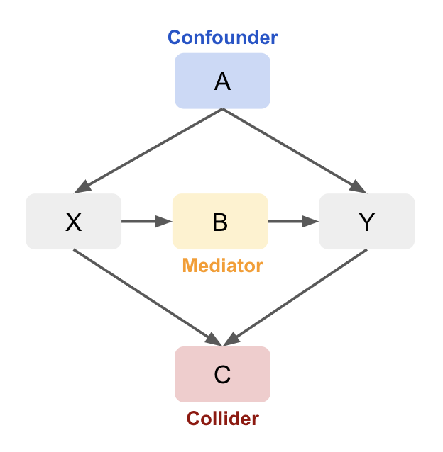
1. Mediator: A variable that lies on the causal path from treatment to outcome, capturing part or all of the effect of treatment.
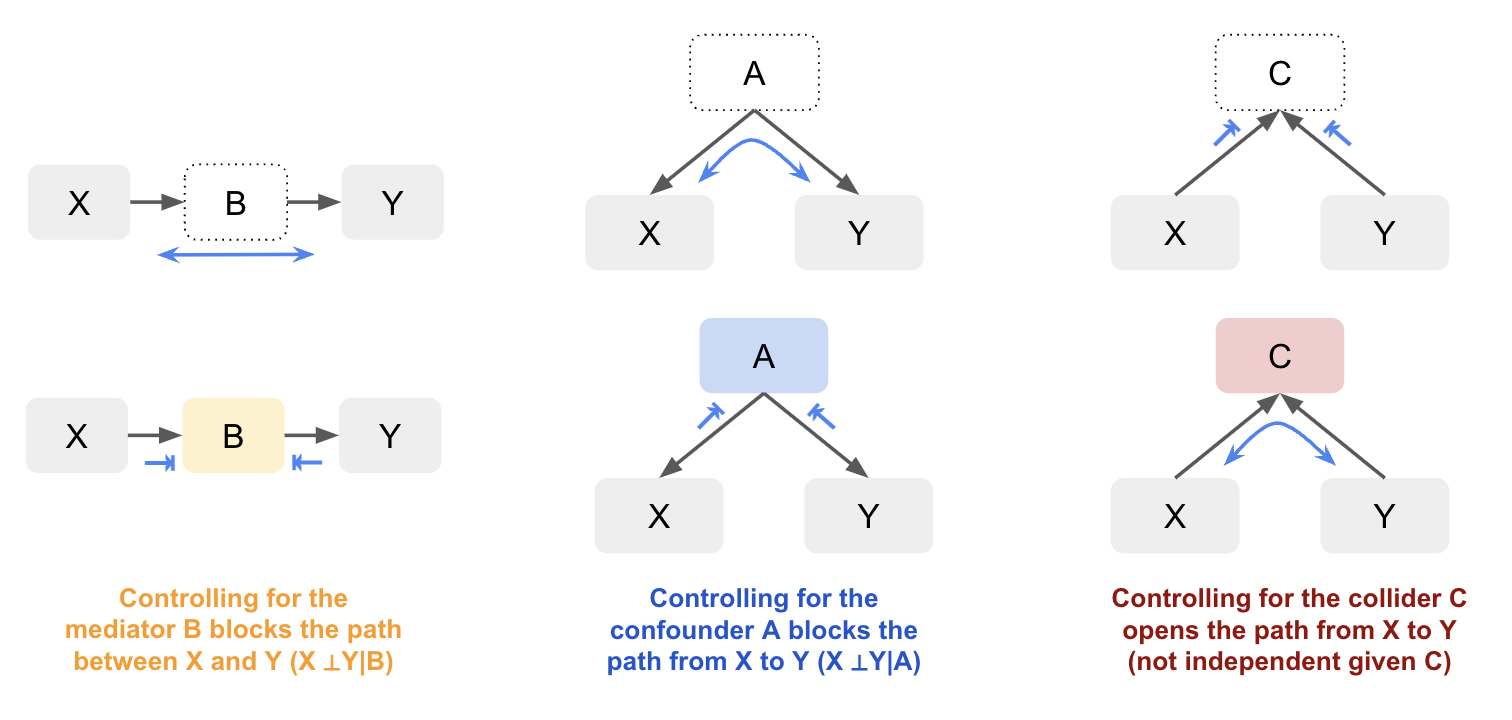
Conditioning on a mediator helps clarify the mechanism by which one variable affects another. Consider a situation where Sales are influenced by both Ad Spend and Web Traffic:
\[\text{Ad Spend} \rightarrow \text{Traffic} \rightarrow \text{Sales}\]Here, increasing Ad Spend increases Traffic, which in turn boosts Sales. If we condition on Traffic, the relationship between Ad Spend and Sales disappears because Traffic fully mediates (explains) this relationship. Mathematically:
\[S \perp \perp A \mid T\]If we fit a regression model without considering traffic, we might mistakenly conclude there’s a direct relationship between ad spend and sales. Once traffic is included, ad spend might no longer be statistically significant, as its effect on sales is mediated by traffic. We might therefore want to optimise ad spend to maximise traffic, using a separate model to predict the effect of the increased traffic on sales. However, if we wanted to estimate the total effect of ad spend on sales, we wouldn’t want to control for traffic as this blocks the indirect path (underestimating the total).
2. Confounder: A variable that causally influences both the treatment and the outcome, potentially introducing spurious correlation if not controlled.
A variable that causes two other variables. Conditioning on this variable is necessary to avoid a spurious association between the two other variables, biasing the causal effect estimate. Imagine that Smoking has a causal effect on both Lung Cancer and Carrying a Lighter:
\[\text{Lighter} \leftarrow \text{Smoking} \rightarrow \text{Lung Cancer}\]While carrying a lighter doesn’t cause lung cancer, if we compare lung cancer rates between people who carry a lighter and those who don’t, we might find a spurious association. This happens because smoking influences both lung cancer and carrying a lighter. To avoid bias, we must condition on smoking, breaking the spurious link between carrying a lighter and lung cancer (\(Lighter \perp \perp Lung Cancer \mid Smoking\)).
In a sales example, if both ad spend and sales increase during the holidays due to seasonality (Ad Spend ← Season → Sales), failing to control for the season could lead to overstating the effect of ad spend on sales.
3. Collider: A variable that is caused by two or more other variables, opening a non-causal path if conditioned on.
Be cautious not to condition on a collider as it can create a spurious relationship between the influencing variables by opening a non-causal path between treatment and outcome (collider bias). In this example, both Ad Spend and Product Quality affect Sales, but they are independent of each other:
\[\text{Ad Spend} \rightarrow \text{Sales} \leftarrow \text{Product Quality}\]Once we condition on sales, we create a spurious association between ad spend and product quality (\(Ad Spend \perp \perp Product Quality\) but \(Ad Spend \not\perp Product Quality \mid Sales\)). When sales are high, both ad spend and product quality may be high, and when sales are low, both may be low. This creates a false impression that ad spend directly improves product quality, even though both only influence sales.
General Rules
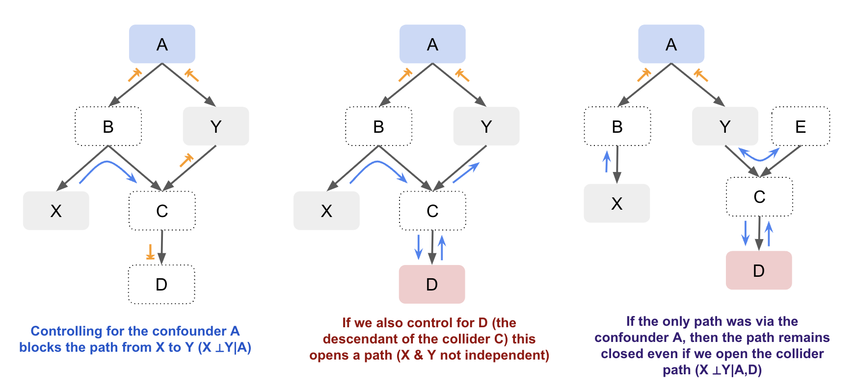
Conditioning on non-colliders (confounders or mediators) blocks the path, making the other variables independent. Conditioning on a collider (or its descendants) creates a dependency between the variables influencing it, which opens the path. Not conditioning on the collider blocks the path, keeping the influencing variables independent.
By visualising causal relationships in a graph, you can better understand how variables are connected and whether observed associations are due to direct causal effects, confounding, mediation, or colliders. By distinguishing between these different relationships, we can handle them appropriately to have more accurate models and inference. While you don’t always need a graph, as the number of variables involved increases it can make it easier to manage. For example, let’s look at just a slightly more complex graph with both confounders and colliders. By visualising the graph it’s easier to identify whether X and Y are independent based on whether there’s an open path between them:
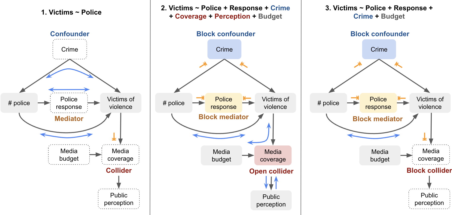
Let’s look at a labelled example. Suppose we want to understand the direct causal relationship between the number of police officers and the number of victims of violent crimes in a city. Depending on what variables we control for, we open different paths and will get different results:
| Model | Variables Included | Notes |
|---|---|---|
1. Victims ~ Police |
Only treatment (Police) | Doesn’t control for confounder (Crime), so may yield biased results (e.g. more police associated with more crime). Mediator (Response) not controlled, so overestimates direct effect. |
2. Victims ~ Police + Response + Crime + Coverage + Perception + Budget |
Treatment, mediator, confounder, and collider path | Opens a backdoor path via collider (Media Coverage), which can create a spurious association between Police and Budget. If both are influenced by a common cause (e.g. City Budget), this can bias the estimate. |
3. Victims ~ Police + Response + Crime + Budget |
Treatment, mediator, confounder, and irrelevant variable | Avoids collider bias by excluding Media Coverage. Including Budget is unnecessary but not harmful unless it reintroduces bias through other unblocked paths. |
Note, if we wanted to measure the total effect of the number of police on the number of victims, we would only control for the confounder in this case, as the mediator would absorbs some or all of the effect.
Systematic bias
Let’s revisit the concept of bias, this time with the help of causal graphs. Systematic bias occurs when an observed association between treatment and outcome is distorted by factors other than the true causal effect. In graphical terms, this often corresponds to open non-causal paths linking treatment and outcome, producing spurious associations even when the true effect is zero (sometimes called bias under the null). Common causes, or confounders, create backdoor paths that induce such spurious associations, while conditioning on common effects, or colliders, opens other non-causal paths and leads to selection bias. Measurement error in confounders or key variables can also contribute by preventing complete adjustment. Additionally, systematic bias can arise from other sources like model misspecification or data issues, which affect the accuracy of effect estimates. In this section, we’ll focus on confounding and collider bias, which can be clearly illustrated using causal graphs.
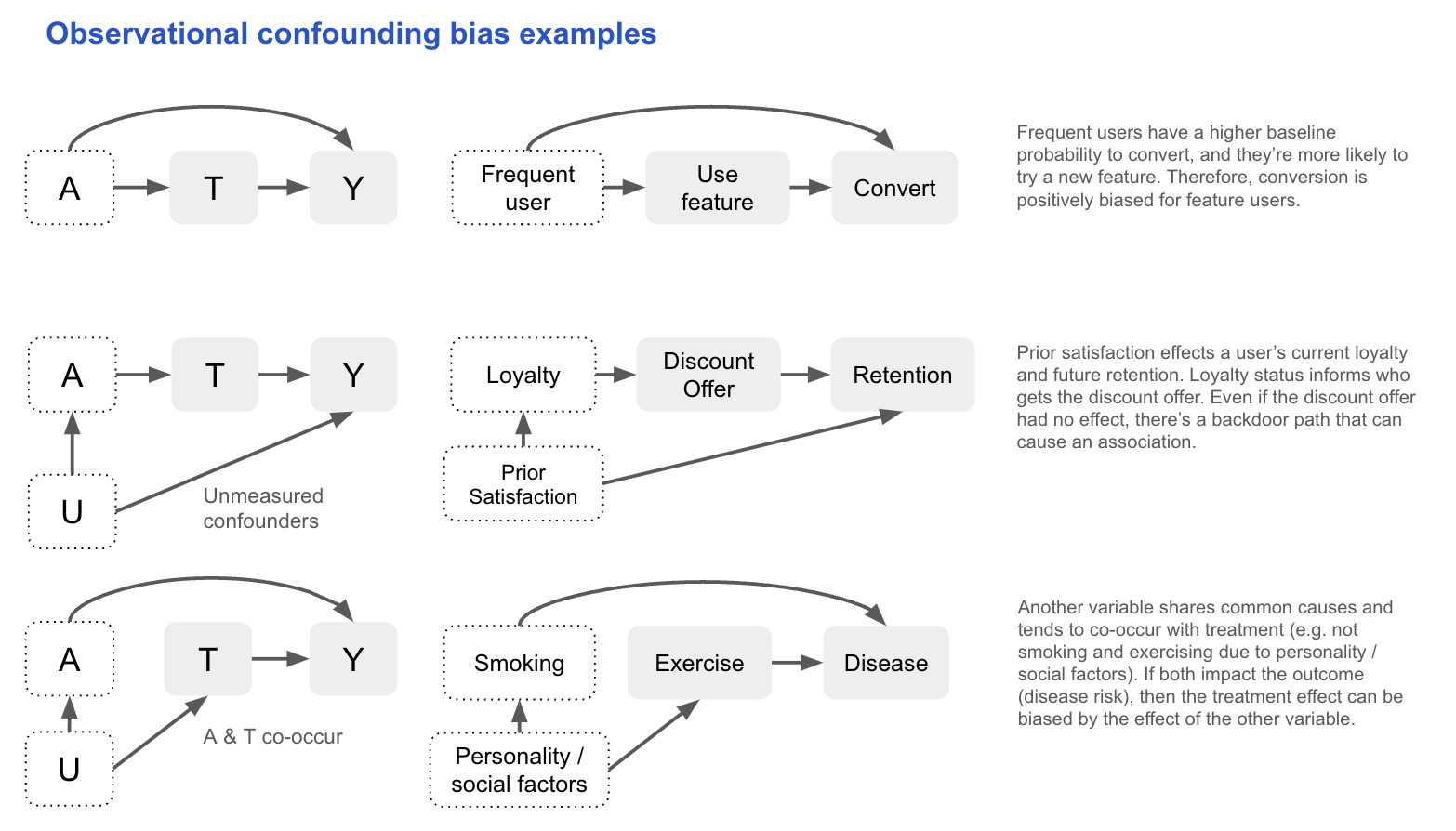
Confounding bias
In observational studies, treatment is not randomised and so it can share causes with the outcome. These common causes (confounders) open backdoor paths between treatment and outcome, creating spurious associations. If you don’t control for them, the observed relationship can reflect both the causal effect of treatment and the effect of these confounders.
If we know the causal DAG that produced the data (i.e. it includes all causes shared by the treatment and outcome, measured and unmeasured), we can assess conditional exchangeability using the backdoor criterion:
All backdoor paths between T and Y are blocked by conditioning on A, and A contains no variables that are descendants of T.
In practice, this assumption is untestable, so we often reason about the likely magnitude and direction of bias:
- Large bias requires strong associations between the confounder and both treatment and outcome.
- If the confounder is unmeasured, sensitivity analysis can test how results change under varying assumptions about its effect size.
- Surrogates for unmeasured confounders (e.g. income for socioeconomic status) can partially reduce bias, though they can’t fully block a backdoor path.
Other methods have different unverifiable assumptions to deal with confounding. Difference-in-Differences (DiD) can be used with a negative outcome control (e.g. pre-treatment value of the outcome) to adjust for confounding. For example, if studying Aspirin’s effect on blood pressure, pre-treatment blood pressure (C) isn’t caused by the Aspirin (A), but shares the same confounders (e.g. pre-existing heart disease). Differences in C between the treatment groups gives us an idea of the bias in the Aspirin–blood pressure (Y) relationship (assuming the confounding effect is the same).
\[E[Y_1 - Y_0 \mid A = 1] = \left( E[Y \mid A = 1] - E[Y \mid A = 0] \right) - \left( E[C \mid A = 1] - E[C \mid A = 0] \right)\]Ultimately, the choice of adjustment method for confounding depends on which assumptions are most plausible. With observational data, uncertainty is unavoidable, so being explicit about assumptions and using sensitivity tests to quantify the potential bias allows others to critically assess your conclusions in a productive way.
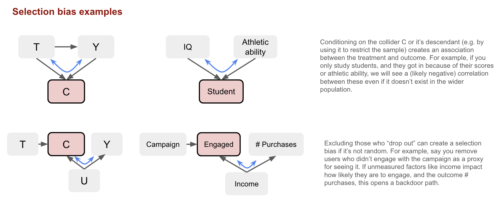
Selection bias
Selection bias refers to bias that arises when individuals or units are selected in a way that affects the generalisability of the results (i.e. it’s not representative of the target population). Here we focus on selection bias under the null, meaning there will be an association even if there’s no causal effect between the treatment and the outcome. This occurs when you condition on a common effect of the treatment and outcome, or causes of each. For example, when observations are removed due to loss to follow up, missing data, or individuals opting in/out:
This can arise even in randomised experiments. Conditional-on-Positives (CoPE) bias occurs when analysis is restricted to “positive” cases for a continuous outcome. For instance, splitting “amount spent” into a participation model (0 vs >0) and a conditional amount model (>0) ignores that treatment can shift people from zero to positive spending. The spenders in treatment and control then differ systematically, and comparing them yields the causal effect plus selection bias
\[E[Y_0 \mid Y_1 > 0] - E[Y_0 \mid Y_0 > 0]\]Typically, control spenders look inflated (negative bias), as those who spend only because of treatment spend less than habitual spenders. We need to account for the fact that treatment affects both the participation decision (whether someone spends anything) and the spending amount (conditional on spending).
Other than design improvements, selection bias can sometimes be corrected with weights (e.g. via Inverse Propensity Weighting). As with confounding, we should also consider the expected direction and magnitude of the bias to understand the impact.
Example: graphs in the wild
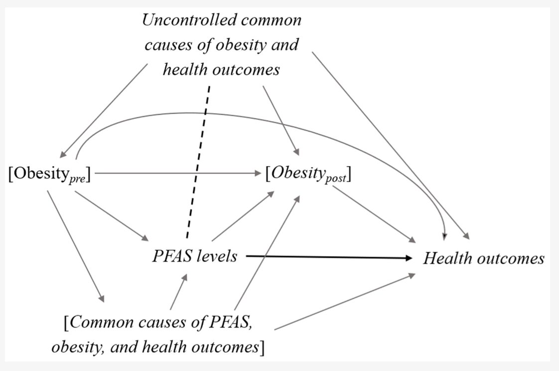
The relationships between variables in causal models can be much more complex in reality, making it challenging to identify the role of each variable. This is especially true when the time ordering of variables is unclear. Let’s consider the graph below looking at the causal effect of PFAS levels on health outcomes, controlling for obesity both before and after exposure:
 Source: Inoue et al., 2020
In the graph, we see a bi-directional relationship between obesity and PFAS levels:
- Pre-obesity (obesity before PFAS exposure) can cause higher PFAS levels because PFAS accumulate in fat tissue. Additionally, obesity itself is associated with worse health outcomes. Therefore, obesity_pre is a confounder because it affects both PFAS levels and health outcomes.
- PFAS exposure may also increase the risk of developing obesity (e.g. due to endocrine disruption or metabolic changes). In this case, obesity_post (obesity after PFAS exposure) is a mediator, as it is part of the causal pathway from PFAS exposure to health outcomes.
- Obesity, PFAS levels, and health outcomes share common causes, such as dietary and lifestyle factors. These factors can affect both obesity and PFAS levels, and so they are also confounders.
To estimate the total effect of PFAS exposure on health outcomes, we want to control for confounders but avoid controlling for mediators, as doing so would block the indirect effect of PFAS on health outcomes via obesity. This is where the issue arises because both obesity and PFAS levels are cumulative measures (i.e. they reflect long-term, prior exposure). Most studies only measure obesity at baseline, and the temporality between PFAS exposure and obesity is not clear. The authors of this graph note that conditioning on obesity_post (post-PFAS exposure) could:
-
- Close the mediating path, thus underestimating the total effect of PFAS on health outcomes; and,
-
- Introduce collider bias, opening a backdoor path between PFAS levels and health outcomes via the uncontrolled common causes of obesity_post (shown by the dotted line in the graph), potentially leading to spurious associations.
They suggest not stratifying on obesity status if it’s likely a mediator of the PFAS-health relationship being studied (as the stratum effects could be biased). On the other hand, it’s generally safe to adjust for the common causes of PFAS and obesity (e.g. sociodemographic factors, lifestyle, and dietary habits) because these factors are less likely to act as mediators in this causal pathway. This is just one example, but it highlights the need to carefully consider the causal graph, and not over-adjust in ways that could bias the causal effects. When you want to measure the total effect, focus on controlling for confounders, not mediators.
Random variability
Random variability (or sampling variability) is the uncertainty that arises because we estimate population parameters using sample data. This is distinct from the sources of systematic bias (confounding, selection, measurement) which are issues of identification.
Statistical consistency
We can think of an estimator as a rule that takes sample data and produces a value for the parameter of interest in the population (the estimand). For example, we calculate the point estimate \(\hat{P}(Y=1 \mid A=a)\) for the population value \(P(Y=1 \mid A=a)\). Estimates will vary around the population value, but an estimator is considered consistent if the estimates get closer to the estimand as the sample size increases. We therefore have greater confidence in an estimate from a larger sample, which is reflected in a smaller confidence interval around it. Note, “consistency” here is a statistical property and different to the identifiability condition which uses “consistency” to mean a well-defined intervention.
Bringing this back to our cake example from earlier: imagine many bakers all trying to bake a cake using the same recipe (estimator). Each baker uses slightly different ingredients or ovens, so their cakes (estimates) vary. However, if you take the average cake quality across many bakers (many samples), that average gets closer to the perfect cake in the cookbook photo (the estimand) as the number of bakers increases. Consistency means that the recipe works on average, with many bakers the results converge to that ideal everyone is aiming for.
To contrast this with bias, now imagine the recipe (estimator) consistently calls for the wrong amount of sugar (i.e. model misspecification). No matter how many bakers try it, their cakes will systematically differ from the perfect cake in the cookbook (the estimand). This persistent deviation is bias, it shifts the average cake away from the target, unlike random variation which only increases the spread (variance) around the true cake. In other words, bias affects the center of the distribution of estimates, while random variability affects its width.
Random variability in experiments
The above is also true in experiments. Random assignment of the treatment doesn’t gaurantee exchangeability in the sample, but rather it means any non-exchangeability is due to random variation and not systematic bias. Sometimes you’re very unlucky and approximate exchangeability doesn’t hold (e.g. you find a significant difference in one or more pre-treatment variables that are confounders).
There’s ongoing debate about whether to adjust for chance imbalances in randomised experiments, particularly for pre-treatment variables that were not part of the randomisation procedure. The basic conditionality principle tells us we can estimate ATE without adjusting for covariates because treatment is randomised (unconfounded), but the extended version justifies conditioning on any pre-treatment X that are not randomised to improve precision (by explaining outcome variance), and estimate sub-group effects (heterogeneity). In practice, a pragmatic approach to avoid aver-adjustment is to adjust only for strong predictors of the outcome that are imbalanced enough to plausibly affect inference.
Confidence intervals
Most methods use standard formulas to calculate standard errors and confidence intervals. In some cases, multiple layers of uncertainty require more advanced techniques, such as bootstrapping, to fully capture all sources of random variability. However, confidence intervals only reflect uncertainty due to random variation; they do not account for systematic biases, whose uncertainty does not diminish as sample size increases.
Summary
Causal inference from observational data relies on strong assumptions to compensate for the lack of randomisation. Identification typically requires three core conditions: consistency (well-defined treatments lead to well-defined outcomes), exchangeability (no unmeasured confounding given observed covariates), and positivity (non-zero probability of treatment across covariate strata). Exchangeability is often the hardest to justify in real-world industry settings. The target trial framework and causal graphs (DAGs) help structure, assess, and communicate these assumptions, as well as the reasoning behind potential sources of bias. Visualising the relationships helps to distinguish what are the mediators, confounders, and colliders, ensuring bias is not introduced when conditioning (or not) on these variables. However, real world graphs can be complex, requiring careful consideration and expert knowledge. In general, you want to avoid over-adjusting, and focus on controlling for confounders.
Data Preparation
Returning to the target trial framework, one of its benefits is that it provides a clear blueprint for data preparation. It forces you to explicitly define: the outcome, target population (eligibility criteria), exposure definition, assignment process, follow up time period, and analysis plan. This helps clarify what data is needed and how it should be processed. In practice, getting to a clean analysis dataset often involves merging multiple sources, engineering features, and resolving issues like time alignment, units, or granularity. Therefore, during this stage, it’s important to run exploratory checks to catch potential problems early, such as:
Measurement error in key variables: Mislabeling treatments or misrecording outcome timestamps can significantly bias results. For example, if some users were marked as having received a notification but never actually did, the estimated treatment effect will be diluted. Similarly, if outcome events are logged with inconsistent timezones or delays (e.g. due to batch jobs), you might misalign treatment and outcome windows. Carefully validating treatment flags and verifying outcome timing logic (especially relative to exposure), can prevent subtle but critical biases.
Missing data: Missingness is rarely random in real-world data. For instance, users who churn stop generating events, resulting in censored outcomes. Or, income data might be missing more often for higher-earning users who opt out of surveys. If the probability of missingness is related to the treatment, outcome, or covariates, ignoring it can introduce bias. It’s important to diagnose the missingness pattern (e.g. checking the proportion missing by variable, treatment and outcome), and consider appropriate handling strategies, such as imputation, modeling dropout, or sensitivity analyses.
This is also a good point to evaluate the identifiability assumptions:
-
Consistency: Are you treating all individuals assigned to the same treatment identically? If there are multiple versions of the “same” treatment (e.g. different types of discounts), this assumption may be violated.
-
Positivity: For every combination of covariates, is there sufficient variation in treatment assignment? In other words, does every subgroup in your data have at least some treated and untreated units? This can be assessed by checking covariate distributions across treatment groups and identifying any zero-probability strata.
-
Exchangeability: This is more difficult to assess directly. It requires that, conditional on observed covariates, treatment assignment is as good as random. We’ll return to this later, as there are method specific diagnostics.
Estimating causal effects with models
So far, we’ve focused on identification: understanding when causal effects can be recovered from observational data under certain assumptions. We now turn to estimation: how to use models to compute those effects in practice. While this section emphasises observational data, the same tools can be applied to randomised experiments (for example, to improve precision by adjusting for covariates).
What is a model?
A model describes the expected relationship between treatment, outcome, and covariates. It defines the conditional distribution of the outcome given these inputs, either through a specified functional form or a flexible algorithm learned from data. In causal inference, models are used to estimate potential outcomes and causal effects under assumptions about the data-generating process.
Many commonly used models are parametric, meaning they assume a fixed functional form. For example, a linear model assumes the expected outcome increases at a constant rate with treatment:
\[E[Y \mid T] = \theta_0 + \theta_1 T\]This is useful when treatment is continuous and the number of observed treatment levels is large or infinite, since the model summarises the effect using only a few parameters. However, to make this work, it must impose strong assumptions like linearity.
In contrast, nonparametric models make fewer assumptions and allow the data to determine the shape of the relationship. Returning to the linear model above, it also serves as a saturated model when treatment \(T\) is binary. In this case, the model estimates two conditional means (one for each treatment group), with no further assumptions. Although written in a linear form, it imposes no constraints and fits the data exactly, making it nonparametric in this specific setting.
Why Models Are Needed
Even if identification assumptions are satisfied, causal effects often can’t be computed directly from raw data. Reasons include:
- High-dimensional covariates: Exact matching becomes infeasible.
- Continuous treatments: Not all treatment levels are observed.
- Sampling variability: Finite data leads to noisy or unstable estimates.
Models help address these challenges. They allow adjustment for covariates (supporting exchangeability), interpolation across treatment levels (helping with positivity), and estimation of potential outcomes under alternative treatment scenarios (relying on consistency). Models can also stabilise estimates by pooling information across similar observations. In this way, modeling isn’t just about computation, it’s how the identifying assumptions are operationalised in practice.
Prediction vs. Inference
Models, by default, describe statistical associations in the observed data; they are not inherently causal. As covered in the introduction to this guide, it’s important to distinguish between using models for prediction (\(E[Y \mid T, X]\)) and for causal inference (\(E[Y(t)]\)). A model may suggest that customers who received a discount spent more, but this observed correlation does not prove the discount caused the increase. Similarly, if you predict bookings based on hotel price without controlling for seasonality, you might incorrectly think increasing the price causes increased demand. In other words, accurately forecasting outcomes does not guarantee valid causal effect estimates.
While predictive models can be evaluated using performance metrics on held-out data, causal inference depends on careful study design and justified assumptions. Specifically, the three identifiability conditions must be met: exchangeability, positivity, and consistency. In addition to these causal assumptions, model-specific assumptions must also hold. For parametric models, these include:
- No measurement error, especially in confounders (an assumption often overlooked but critical for validity); and,
- Correct functional form, meaning the model accurately reflects the underlying data-generating process (no misspecification).
Since all models simplify reality, some degree of misspecification is inevitable. This makes sensitivity analysis essential for assessing how results change under alternative settings. Transparency about assumptions and rigor in testing their robustness help build confidence in the resulting causal estimates.
Extrapolation
A risk with models like regression is it introduces the possibility of extrapolation. Interpolation refers to estimating outcomes within the range of observed data and is generally safe. Extrapolation occurs when making predictions outside the support of the data. For example, estimating effects for treatment levels or covariate profiles that are rare or unobserved. This relies entirely on model assumptions and can lead to misleading results. In causal inference, extrapolation should be avoided unless supported by strong domain knowledge.
Common ATE models
The following sections will go through some of the common models used to estimate the ATE, including:
1. Adjustment-Based Methods: These rely on adjusting for observed confounders to identify causal effects.
- Outcome regression (GLMs): Estimate the expected outcome given treatment and covariates using models such as linear or logistic regression.
- G-computation (standardisation / g-formula): Estimate causal effects by modeling the full outcome distribution under each treatment regime. These are especially useful for longitudinal or time-varying treatments.
- Matching methods: Compare treated and untreated units with similar covariates or scores to mimic a randomised experiment.
- Propensity score methods: Balance covariates between treated and untreated groups before estimating effects.
- Orthogonal machine learning (Orthogonal ML): Combine machine learning with causal assumptions to reduce bias and improve robustness.
2. Quasi-Experimental Designs: These exploit natural experiments or design features to identify causal effects without relying solely on observed confounding adjustment.
- Instrumental Variable (IV) analysis: Uses external variation that influences treatment but not directly the outcome to handle unmeasured confounding.
- Difference-in-Differences (DiD): Compares changes over time between treated and control groups in panel data.
- Two-Way Fixed Effects (TWFE): A panel data regression approach extending DiD with multiple groups and time periods.
- Synthetic Control Methods: Construct a weighted combination of control units to approximate the treated unit’s counterfactual.
- Bayesian Structural Time Series (BSTS): A Bayesian approach to estimate causal impacts in time series, often used in policy evaluation.
- Regression Discontinuity Designs (RDD): Leverages treatment assignment cutoffs to estimate local causal effects near the threshold.
Each of these methods builds on the core identification assumptions but uses different strategies to estimate causal effects, depending on the data structure, assumptions, and sources of bias. There is no one size fits all approach, as most methods are designed for a narrow set of conditions. Therefore, it’s useful to be familiar with a range of approaches, and go deeper in those most relevant to your use case.
Adjustment based methods
Outcome regression
Generalised Linear Models (GLMs) such as linear regression are a popular choice for estimating ATE when there isn’t complex longitudinal data. For example, using a binary variable to indicate whether an observation was treated or not (T), for a continuous outcome we get:
\[Y_i = \beta_0 + \beta_1 T_i + \epsilon_i\]Where:
- \(\beta_0\) is the average Y when \(T_i=0\) (i.e \(E[Y \mid T=0]\))
- \(\beta_0 + \beta_1\) is the average Y when \(T_i=1\) (i.e. \(E[Y \mid T=1]\))
- \(\beta_1\) is therefore the difference in means (i.e. \(E[Y \mid T=1] - E[Y \mid T=0]\))
- \(\epsilon\) is the error (everything else that influences Y)
In this single variable case, the linear regression is computing the difference in group means. If T is randomly assigned then \(\beta_1\) unbiasedly estimates the ATE:
\[ATE = \beta_1 = \frac{Cov(Y_i, T_i)}{Var(T_i)}\]However, when using observational data, the key assumption of exchangeability often fails (\(E[Y_0 \mid T=0] \neq E[Y_0 \mid T=1]\)). To address this, we can extend the model to control for all confounders \(X_k\) (i.e. variables that affect both treatment and outcome):
\[Y_i = \beta_0 + \beta_1 T_i + \beta_k X_{ki} + \epsilon_i\]Now \(\beta_1\) estimates the average treatment effect (difference in group means), conditional on the confounders (i.e. the conditional difference in means). Under linearity and correct model specification, this equals the marginal ATE (population-average ATE).
To break this down, you can imagine we instead did this in 2 steps: 1) regress T on X to isolate the variation in T not explained by the confounders (i.e. the residuals, which are orthogonal to X by design); 2) regress Y on the residuals from step 1 (the part of T that isn’t explained by X). If T was randomised, then X would have no predictive power and the residuals would just be the original T. Conceptually, we’re isolating the variation in treatment assignment that is unrelated to confounders (the residuals), and then estimating how this variation relates to the outcome to isolate the treatment effect net of confounding.
The normal equation does this in one step for multiple regression using the inverse matrix (\(\left(X^\top X\right)^{-1}\)) to “adjust” each predictor’s covariance with Y for the correlations among the predictors.
Considerations
Model assumptions
When using linear regression to estimate the ATE, the most important model assumptions are correct functional form (linearity in parameters) and no unmeasured confounding (exogeneity: X is not correlated with the error term), because violations of these lead to biased and inconsistent estimates of the treatment effect. These can be partially assessed by inspecting residual plots, adding interaction or nonlinear terms, and relying on domain knowledge to ensure all major confounders are included.
The other assumptions concern the errors and primarily affect inference rather than the point estimate: independence of errors, homoscedasticity (constant variance of the errors), and normality (in small samples). Violations can distort standard errors and confidence intervals, impacting our ability to quantify uncertainty around the ATE. Standard approaches to address these include using robust or cluster-robust standard errors, transforming variables, or modeling correlations in clustered or time-series data.
Avoid over-adjusting
To have an unbiased estimate we need to include all confounders in the model. However, this is often the most challenging aspect when working with observational data in industry settings. Unless you have a tightly controlled process with well-understood and measured mechanisms, some unmeasured confounding is likely to remain. It can be tempting to include every available variable to “adjust as much as possible,” but over-adjusting can actually introduce bias or increase variance, reducing the power to detect the true effect. Therefore, it’s important to be deliberate in choosing which variables to include:
✅ Predictors of the outcome: Including variables that predict the outcome helps reduce unexplained variation (noise) and improves the precision of the treatment effect estimate.
❌ Pure predictors of the treatment: These variables affect treatment assignment but have no relation to the outcome. Including them can reduce the variation in treatment, inflating standard errors and reducing power, though they do not bias the estimate if unrelated to the outcome.
❌ Mediators: Variables that lie on the causal pathway from treatment to outcome. Controlling for mediators blocks part of the treatment effect, causing underestimation of the total effect.
❌ Colliders: Variables influenced by both treatment and outcome (or their causes). Conditioning on colliders opens a backdoor path and induces spurious associations, biasing the estimate. For example, controlling for job type when estimating the effect of education on income may introduce bias because job type is affected by both education and income.
It’s worth mentioning one common mistake: using variable selection methods from predictive modeling to select confounders (e.g. step-wise methods or regularisation). A variable’s ability to predict the outcome (an association) does not tell us whether it’s a confounder. Therefore, blindly applying automated variable selection methods is a bad idea. Confounding is about relationships with both the treatment and the outcome, so variable selection for causal models must be grounded in domain knowledge and causal reasoning.
Implicit weighting
Coming back to our example of estimating ATE using $\beta_1$ from \(Y = \beta_0 + \beta_1 T + \beta_k X_{k}\). This effectively estimates treatment effects within each subgroup (stratum) defined by $X$, then averages those subgroup effects. However, the implicit weights assigned to each subgroup depend not just on subgroup size, but on the amount of treatment variation within that subgroup. Subgroups with more treatment variation provide more information for estimating $\beta_1$, so the model gives them more influence in order to minimise prediction error.
Mathematically, $\hat{\beta}_1$ is a weighted average of subgroup-specific treatment effects:
\[\hat{\beta}_1 = \sum_{s} w_s \hat{\beta}_{1,s}\]Where $s$ indexes subgroups, $\hat{\beta}_{1,s}$ is the treatment effect in subgroup $s$, and the weights $w_s$ are proportional to:
\[w_s \propto \text{Var}(T \mid X = s) \times n_s\]Here, $n_s$ is the size of subgroup $s$, and $\text{Var}(T \mid X = s)$ is the variance of treatment within subgroup $s$ (e.g. for binary treatment it would be $p_s(1-p_s), where $p_s$ is the treated proportion in subgroup s). This means that subgroups with limited treatment variation (small $\text{Var}(T \mid X = s)$) get very little weight, even if large in size.
For example, suppose $X$ indicates platform type: 800 mobile users (790 treated, 10 control), and 200 desktop users (100 treated, 100 control). The true treatment effect is 1 for mobile users and 2 for desktop users. Even though mobile users are 80% of the sample, their near-complete lack of treatment variation means the constant-effect regression places most weight on the desktop subgroup, resulting in an estimate closer to 2, instead of the true population weighted ATE: $0.8 \times 1 + 0.2 \times 2 = 1.2$.
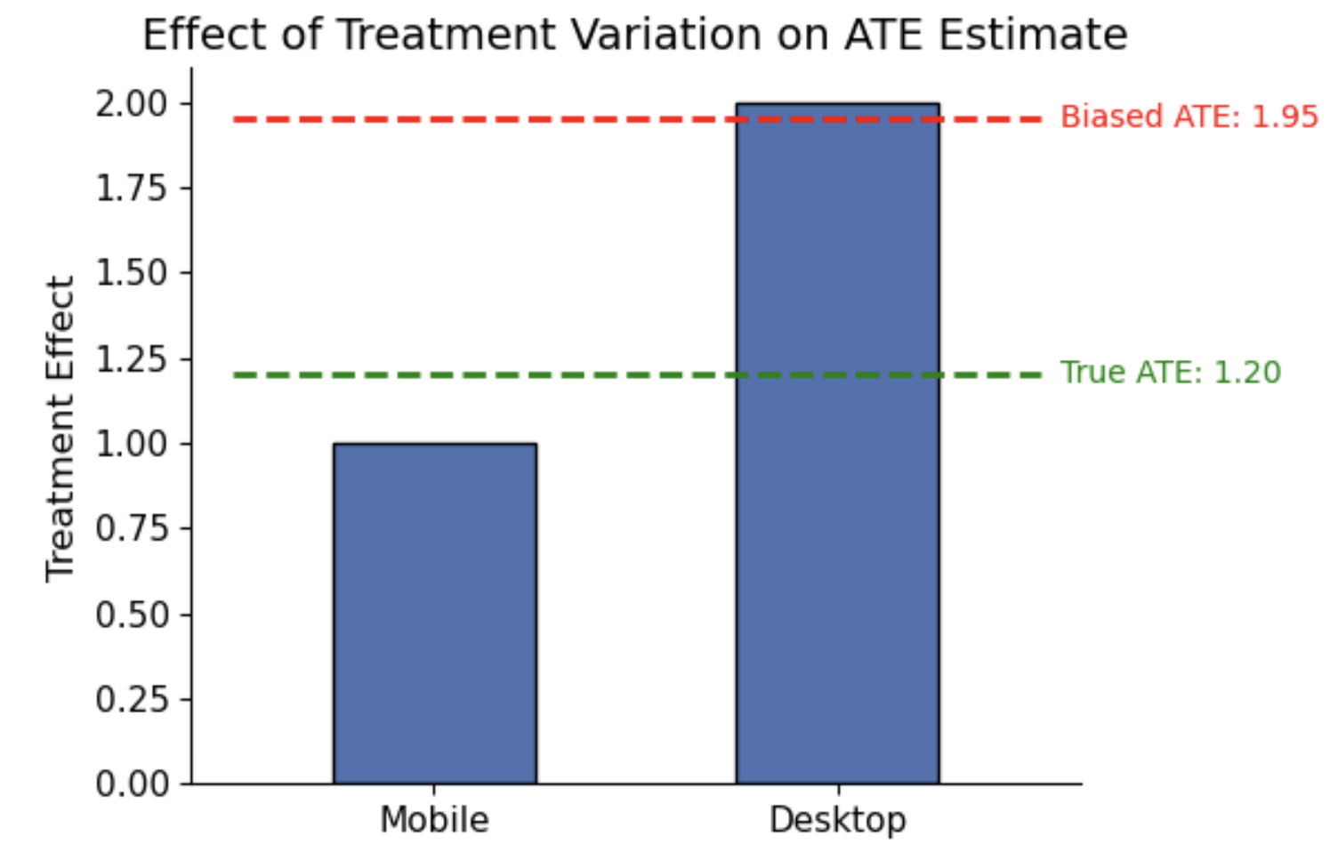
This issue is a model misspecification: forcing a constant treatment effect means the regression compromises on a slope that fits the high-overlap subgroup best, even if it misrepresents the true ATE. Specifically, bias arises when:
- X affects T (i.e. treatment variation differs by subgroup, such as 80/20 in group 1 but 50/50 in group 2); and,
- X affects Y, either by changing baseline outcomes (e.g. desktop users purchase more even without treatment), or by moderating the treatment effect (e.g. desktop users gain +4 pp from treatment, mobile users only +1 pp).
If X does not affect Y, treatment effect is constant across subgroups, so the ATE estimate is unbiased even if there’s differences in treatment variation. Conversely, if X affects Y by moderating the treatment effect (i.e. heterogeneous effects), but treatment variation is equal across subgroups (i.e. $X$ does not affect $T$ = equal T/C split), the regression’s implicit weights match subgroup sizes, and the ATE is unbiased.
When positivity is violated or nearly violated (i.e. some subgroups are mostly treated or control), this misspecification worsens. To fit a single slope, the model extrapolates into regions of X with no treated or control units. In linear models, this can produce negative weights, effectively counterbalancing influence from data-rich regions with “imaginary” influence from unsupported regions, leading to unstable and potentially biased ATE estimates.
Practical checks:
- Inspect treatment balance within subgroups of $X$ to identify poor overlap.
- If overlap is insufficient, consider reporting subgroup-specific effects instead of a single ATE, and restrict analysis to regions of $X$ with adequate overlap.
- Examine implied weights, for example using the lmw package in R, based on Chattopadhyay & Zubizarreta (2023).
Correctly estimating ATE with heterogeneous effects:
To properly estimate the ATE in the presence of heterogeneity (and treatment variation), you can explicitly model interactions between treatment and covariates (e.g. $T \times X$ terms). This allows the regression to estimate a separate treatment effect for each subgroup. Then, use g-computation (covered in more detail in the next section) to recover the population ATE:
- Fit the interaction model on the observed data.
- For each individual, predict their outcome twice: once setting $T=1$ and once setting $T=0$ (while keeping $X$ at its observed values).
- Compute the individual-level differences between these two predictions.
- Average these differences across the sample to obtain the ATE.
This approach ensures the ATE reflects subgroup effects weighted by population prevalence, while adjusting for confounding.
Continuous treatments
This framework also applies when the treatment T is continuous, such as dosage, time spent on a feature, or monetary exposure. In that case, \(\beta_1\) is interpreted as a marginal effect: the expected change in outcome Y for a one-unit increase in treatment T (assuming a constant effect), holding covariates X constant. The same assumptions are required, but using linear regression imposes a constant treatment effect across the entire range of T. If the true relationship is nonlinear, this can lead to biased or misleading estimates.
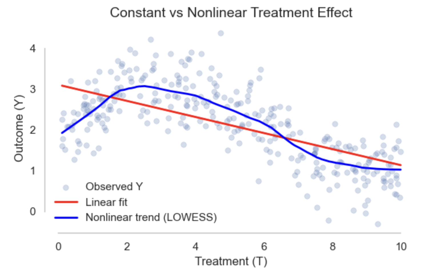
When the treatment effect varies across it’s range like in the example above, more flexible models may be needed (e.g. splines, GAMs, or kernel regression). To estimate the ATE, you then use standardisation (g-computation): compute the predicted outcomes at different treatment levels for each unit, and average the difference across the population. This gives you a robust estimate of the average effect, even when the treatment effect is not constant, and can be combined with bootstrapping to get confidence intervals.
Binary outcomes
For binary outcomes, linear regression is still commonly used (known as Linear Probability Models, LPM), especially when the goal is to estimate the ATE on the probability scale. The model is fitted just like before, but because the outcome is binary, there are important differences in interpretation and limitations. Specifically, $\beta_1$ estimates the difference in outcome probabilities between treated and untreated groups (the ATE on the probability scale). The model assumes a constant marginal effect, meaning treatment shifts the probability by the same amount for everyone, regardless of their baseline risk. This can oversimplify reality if effects vary across individuals.
LPMs have other practical drawbacks: they can predict probabilities outside the $[0,1]$ range, and the variance of residuals depends on the predicted probability (heteroskedasticity), peaking around 0.5. This violates ordinary least squares (OLS) assumptions, potentially distorting standard errors. Therefore, it is important to use robust (heteroskedasticity-consistent) standard errors and be cautious when predicted probabilities are close to 0 or 1.
If more accurate modeling of the relationship between covariates and the outcome is needed, especially for prediction or rare outcomes, logistic regression is often preferred. However, logistic regression coefficients represent log-odds ratios rather than probability differences, so $\beta_1$ is not directly interpretable as the ATE. This is because logistic regression models a latent continuous propensity that is squashed by the logistic function. The same absolute change in probability corresponds to different changes in log-odds depending on the covariate values and residual variation. Consequently, the log-odds coefficient for treatment does not directly equal the probability difference between treated and untreated groups.
To recover the ATE on the probability scale, two common methods are:
-
Average Marginal Effects (AME): For each observation, compute the marginal effect of treatment:
\[\text{ME}_i = \hat{P}_i \times (1 - \hat{P}_i) \times \hat{\beta}_1\]Where $\hat{P}_i$ is the predicted probability for individual $i$. The AME is the average of these marginal effects across all observations. Intuitively, you can think of the logistic function as a hill: the slope (marginal effect) varies depending on where you stand (the covariates). Some individuals are near the hilltop or base, where the slope is flat, and others are on the steep middle slope. By averaging everyone’s slope, the AME summarises the average steepness of the hill: the average effect of treatment on the probability scale.
-
Marginal Standardisation (g-computation): After fitting the logistic model, predict each individual’s outcome twice: once with $T_i = 1$ and once with $T_i = 0$, while keeping covariates $X_i$ fixed at their observed values. The ATE is:
\[\text{ATE} = \frac{1}{n} \sum_{i=1}^n \left[ \hat{Y}_i(T=1) - \hat{Y}_i(T=0) \right]\]This represents the average difference in predicted probabilities if everyone were treated versus if no one were treated. In single-time-point settings, this is equivalent to g-computation (covered in the next section).
For both methods, standard errors can be estimated using the Delta method or bootstrapping. The Delta method provides a fast, analytic approximation based on a Taylor expansion, while bootstrapping offers a flexible approach that is often more robust, particularly in complex models or small samples.
Causal strength
Assuming the model is specified correctly, the reliability of outcome regression for causal inference hinges on the validity of the identifiability assumptions:
- Exchangeability (no unmeasured confounding): Conditional on covariates X, the treatment assignment is as good as random. Violations result in omitted variable bias. This is not a testable assumption as we can never be sure all confounders are measured and correctly included.
- Positivity (overlap): Positivity requires that for every combination of covariates X, there is a non-zero probability of receiving both treatment and control. This ensures that we can make meaningful comparisons between treated and untreated units within every subgroup of X. Violations result in extrapolation as regression models predict effects for units outside the support of the data, which can be unreliable. Pre-processing to restrict the population of interest might be possible, though it limits generalisability.
- Consistency: The treatment is well-defined and uniformly applied. Violations lead to ambiguity about what effect is being estimated, weakening causal interpretation. This can be more challenging with observational data, with violations potentially being more hidden when regression is used (e.g. controlling for post-treatment variables could remove part of the treatment effect).
G-computation (standardisation)
G-computation (also known as standardisation and the g-formula), takes a different approach to effect estimation. The “g” stands for generalised, as in the generalised formula for computing causal effects from observational data. Instead of relying on the treatment coefficient from a regression model, it explicitly estimates each individual’s potential outcomes under treatment and control, and then averages them to compute the average treatment effect (ATE):
-
Fit an outcome model Estimate $\hat{Y}(T, X)$, a model for the outcome $Y$ as a function of treatment $T$ and covariates $X$. This is typically a parametric model (e.g. linear or logistic regression), although more flexible models can also be used.
-
Predict potential outcomes For each observation $i$, use the fitted model to predict:
- $\hat{Y}_i(1) = \hat{Y}(T=1, X_i)$: the predicted outcome if treated
- $\hat{Y}_i(0) = \hat{Y}(T=0, X_i)$: the predicted outcome if not treated
This simulates both counterfactual outcomes for each individual.
-
Compute the ATE
Average the individual level differences to get the ATE:
\[\widehat{ATE} = \frac{1}{n} \sum_{i=1}^n \left( \hat{Y}_i(1) - \hat{Y}_i(0) \right)\]The target estimand (e.g., ATE, ATT) is explicit, because you define it through the population over which you average the potential outcomes.
If the outcome model is linear and assumes a constant treatment effect, such as \(Y = \beta_0 + \beta_T T + \beta_X^\top X + \varepsilon\), then standardisation will produce the same ATE estimate as you’d get from $\hat{\beta}_T$. This is because the predicted difference for each individual is: \(\hat{Y}_i(1) - \hat{Y}_i(0) = \hat{\beta}_T\). However, this equivalence holds only under a linear model with no effect heterogeneity (i.e. constant treatment effect), and when the model is correctly specified.
Benefits
The key benefit is it generalises beyond linear models:
- Allows for non-linear relationships, interactions, or flexible ML models;
- Makes the estimand explicit: you’re computing the mean of potential outcomes, not just interpreting a coefficient
- Lets you easily compute subgroup effects (e.g. the ATT) by averaging over specific subsets
- Provides an intuitive link between observed data and potential outcomes
However, it shares the same core vulnerability as any modeling-based method: if the outcome model is misspecified, the causal estimates can be biased.
Using ML models
While it’s traditionally associated with parametric outcome models (like linear or logistic regression), the method itself is model agnostic. Any model that predicts $\hat{Y}(T, X)$ well can be used, including machine learning approaches that can better capture non-linear relationships and interactions in the data. However, increased model flexibility comes with some risks:
- ML models can overfit, especially in small data or high-dimensional settings
- They may extrapolate poorly in regions with little data (especially with poor treatment overlap)
- Their predictions may be miscalibrated, leading to systematic bias in estimating potential outcomes
Since the final causal estimate is computed by averaging these predicted potential outcomes, some individual-level prediction errors may cancel out. However, systematic biases, especially those that differ by treatment group, can lead to biased estimates of the treatment effect. To mitigate these risks:
- Use out-of-sample predictions (e.g. via cross-validation)
- Check for treatment group overlap, and avoid extrapolating to unsupported regions
- Consider separate models for treated and control groups if treatment effects vary or the groups are imbalanced
- Tune complexity to avoid over-regularisation (strong regularisation, such as in Lasso or tree pruning, may improve prediction but introduce bias in treatment effect estimation)
While ML models offer flexibility and the ability to model complex relationships, they often come at the cost of reduced interpretability. Therefore, rigorous validation, both predictive and causal, is essential.
Confidence intervals
The simulation-like steps of g-computation create multiple layers of uncertainty (estimating the outcome model, predicting potential outcomes, then averaging them). Given this complexity, there’s often no closed-form expression for the standard error of the treatment effect estimate.
However, in certain cases, namely when the outcome model is linear and we assume a constant treatment effect, a closed-form solution is available using the Delta method. Under a linear model (e.g., $Y = \beta_0 + \beta_T T + \beta_X^\top X$), the predicted outcomes under treatment and control differ only in the coefficient on $T$, so:
\[\hat{Y}_i(1) - \hat{Y}_i(0) = \hat{\beta}_T\]The standard error of the ATE is just the standard error of $\hat{\beta}_T$, and a 95% confidence interval can be constructed as:
\[\hat{\beta}_T \pm 1.96 \cdot \text{SE}(\hat{\beta}_T)\]In more realistic settings where treatment effects vary and outcome models are flexible or nonlinear, we use resampling methods to quantify uncertainty:
-
Bootstrapping is the most common approach. It involves repeatedly resampling the data, refitting the outcome model, predicting potential outcomes, and recomputing the treatment effect. The variability across bootstrap estimates is used to construct percentile-based or bias-corrected confidence intervals.
-
Cross-fitting (or sample splitting) can reduce overfitting bias when using machine learning. Out-of-fold predictions are used to estimate potential outcomes, and variance is estimated across folds. Cross-fitting is often used alongside bootstrap.
Causal strength
G-computation relies on the assumption that the outcome model is correctly specified and sufficiently flexible to capture the true relationship between treatment, covariates, and outcome. Mis-specification or poor fit can bias results, especially in regions with sparse data or complex interactions. Using flexible machine learning models can help address this, but it requires careful model tuning, diagnostics, and validation. If this holds, it provides a transparent and interpretable way to estimate causal effects by simulating counterfactual outcomes.
The key identifiability assumptions for valid causal inference still remain:
- Exchangeability (No unmeasured confounding): All confounders affecting both treatment and outcome must be observed and properly included in the model. Violations cause bias due to omitted variables.
- Positivity (Overlap): Every individual has a positive probability of receiving either treatment or control given their covariates. Lack of overlap leads to extrapolation beyond the data, resulting in unstable or biased estimates.
- Consistency: The treatment must be well-defined and consistently applied, so that the potential outcomes correspond to well-specified interventions.
Matching
Matching tries to approximate a randomised experiment by directly comparing similar observations. Meaning for each treated observation, we’re looking for a similar (exchangeable) untreated observation to compare to based on some set of covariates X. Unlike regression which adjusts for covariates in estimation, matching first selects a balanced subset of the data based on the covariates and then does a direct comparison. Exact matching, where matched units share identical covariate values, quickly becomes infeasible as the number of covariates grows or when covariates are continuous. Therefore, approximate matching methods are more common. This requires us to define a measurement of proximity (distance) to select the “closest” matches. For example, nearest neighbor matching pairs treated units with untreated units based on a distance metric such as Euclidean or Mahalanobis distance.
Other methods not covered here include propensity score matching (in the next section), and optimal or genetic matching. Matching is naturally suited for estimating ATT, because it uses the treated group as the reference and finds comparable controls. However, we can approximate ATE with bi-directional matching for both the treated and control group.
Distance measures
Matching identifies untreated units closest to each treated unit using a distance metric over covariates. The choice of metric affects covariate balance and thus the credibility of treatment effect estimates. Common choices include Mahalanobis, Euclidean, and propensity score distances (discussed in the next section).
Mahalanobis distance
Mahalanobis distance measures how far apart two points are in a multivariate sense, accounting for both the scale of each covariate and the relationships (correlations) between covariates. This prevents variables with large variance or high correlation from dominating the matching. It’s especially useful when matching on multiple continuous covariates. The distance between treated and control units is computed using the inverse covariance matrix of the covariates:
\[d(i, j) = \sqrt{(X_i - X_j)^\top S^{-1} (X_i - X_j)}\]Where:
- $X_i$ and $X_j$ are the covariate vectors for units $i$ and $j$
- $S$ is the sample covariance matrix of the covariates (computed across all units in the control group, or the full sample if distributions are similar)
- $S^{-1}$ is the inverse of the covariance matrix
This rescales the differences between covariates based on their variance and correlation structure. Differences on variables with high variance count less, and correlated covariates are downweighted to avoid double-counting shared information. The calculation can be broken down as:
-
Multiply the inverse covariance matrix $S^{-1}$ by the difference vector $X_i - X_j$ to get a transformed vector that weights each variable’s difference according to its variance (diagonal entries) and correlations with other variables (off-diagonal entries). Variables with high variance have smaller diagonal values in $S^{-1}$, so differences contribute less to the total distance. The off-diagonal entries adjust for correlated variables, downweighting differences aligned with expected correlations (e.g., height and weight moving together), while differences orthogonal to those correlations (unexpected variation) are upweighted.
-
Multiply the result from step 1 by the transpose of the difference vector to obtain a scalar measuring the weighted squared distance between the two points. Taking the square root converts this into the Mahalanobis distance.
Euclidean
Euclidean distance is the simplest and most intuitive way to measure similarity between two units based on their covariates. It calculates the straight-line distance between points in multidimensional space by treating each covariate as a dimension. Specifically, it computes the difference between each covariate for units i and j, squares these differences, sums them, and takes the square root:
\[d(i, j) = \sqrt{(\mathbf{X}_i - \mathbf{X}_j)^\top (\mathbf{X}_i - \mathbf{X}_j)}\]Because it relies on squared differences, variables with larger scales or ranges can dominate the distance calculation. Therefore, standardizing or normalizing covariates beforehand is common practice to ensure each covariate contributes proportionally. Another limitation is that Euclidean distance assumes covariates are independent and uncorrelated, which may not hold in practice, potentially leading to less optimal matches compared to methods like Mahalanobis distance. Despite this, its simplicity and computational efficiency make it a good choice when covariates are on similar scales and roughly uncorrelated.
Binary / categorical variables
Binary variables are typically treated as numeric (0/1) and included directly in distance calculations. This generally works well when the variables are balanced and consistently coded. For Euclidean distance, binary variables should be scaled or normalized with other covariates to prevent them from disproportionately influencing the distance. For Mahalanobis distance, scaling is implicit via the covariance matrix; however, when categories are rare, the covariance matrix can become unstable or near-singular, which requires inspection and possibly corrective action (e.g., grouping rare categories).
Categorical variables are usually handled by one-hot encoding each category into separate binary variables, which can then be treated like binary variables in distance computations. When certain categorical variables are critical confounders, exact matching or coarsened exact matching (grouping categories into broader bins) may be preferred to ensure treated and control units are matched exactly or approximately on these variables. This helps avoid imbalance that could bias causal estimates.
If rare categories or small sample sizes threaten the stability of the covariance matrix or matching quality, combining levels (coarsening) or using alternative distance measures may be appropriate (e.g. Gower distance computes a scaled distance per variable, handling different data types, then averages them).
Neighbor matching
Once we have a measure of distance $d(i,j)$, we match each treated unit to control unit(s) with the smallest distance. After sorting the distances $d_{ij}$ for all control units $j$ relative to treated unit $i$, we can select one or more matches:
- Nearest neighbor matching: Matches each treated unit to the single control unit with the smallest distance. It’s simple and intuitive but can risk poor matches if the closest control is still quite different.
- K-nearest neighbor matching: Matches each treated unit to the top $k$ closest control units. This reduces variance by including more controls but may incorporate less similar matches if $k$ is large.
Matching is often performed with replacement, allowing a control unit to be matched multiple times to different treated units. This tends to improve match quality and reduce bias, especially when treatment and control groups are imbalanced. However, matching with replacement can inflate variance and overuse certain control units. In settings where groups are large and well-balanced, matching without replacement may be preferred, or a limit might be set on the number of matches per control.
Caliper restriction
Caliper matching is a refinement of nearest neighbor matching that restricts matches to only those control units whose distance to the treated unit is within a specified threshold, called the caliper. The caliper sets a maximum acceptable distance between matched units, ensuring that matches are sufficiently close and thereby improving the quality of matches (reducing bias). However, there is a bias-variance trade-off: if the caliper is too small, it can exclude many treated units, reducing sample size and statistical power; and, too large risks including poor matches, increasing bias. Typically you would start with recommended defaults (e.g. 0.2 standard deviations), then assess the covariate balance (see the next section) and sample retention (might be losing generalizability and precision), iteratively adjusting as needed.
Estimating the treatment effect
After matching, several common estimators can be used to calculate treatment effects from matched data.
1. ATT via Treated Matching
The average treatment effect on the treated (ATT) is estimated as:
\[\widehat{ATT} = \frac{1}{N_T} \sum_{i \in T=1} \left( Y_i - \frac{1}{M_i} \sum_{j \in \text{matched}(i)} Y_j \right)\]For each treated unit $i$, subtract the average outcome of its $M_i$ matched control units $j$. Only treated units contribute to this estimator. Matching can be performed with or without replacement. Standard errors can be estimated using bootstrapping to account for the dependence induced by matching.
2. Symmetric Matching
The average treatment effect (ATE) can be estimated via 1-to-1 symmetric matching:
\[\widehat{ATE} = \frac{1}{N} \sum_{i=1}^{N} (2T_i - 1)\left(Y_i - Y_{jm(i)}\right)\]Each unit $i$ is matched to exactly one unit $jm(i)$ from the opposite treatment group. The term $(2T_i - 1)$ equals $+1$ for treated units and $-1$ for controls, ensuring differences $Y_i - Y_{jm(i)}$ are consistently signed as treated minus control outcomes. All $N = N_T + N_C$ units contribute once, making the estimator symmetric. This approach works best when treatment and control groups are balanced and have good overlap.
3. ATE via Reweighting
A more general ATE estimator that accounts for asymmetry in matching or reuse of units is:
\[\widehat{ATE} = \frac{1}{2} \left[ \frac{1}{N_T} \sum_{i \in T=1} \left( Y_i - \frac{1}{M_i} \sum_j Y_j \right) + \frac{1}{N_C} \sum_{j \in T=0} \left( \frac{1}{M_j} \sum_i Y_i - Y_j \right) \right]\]This combines the ATT for treated units matched to controls and the ATC for control units matched to treated units. By weighting both groups equally, it estimates the full ATE even when the groups are imbalanced. Bootstrapping is recommended for standard errors due to the dependence created by matching.
All of these approaches approximate the ATE under strong overlap (positivity) and good covariate balance. When treatment assignment is highly imbalanced, ATT or ATC may be more reliable than the symmetric or reweighted ATE. To summarise:
- ATT: Focuses only on treated units, comparing each to its matched controls. Useful when the treated group is the primary target.
- Symmetric Matching: Treats treated and control units equally in 1-to-1 matches. Good for balanced datasets.
- Reweighted ATE: Combines both perspectives, weighting treated and control units equally, accommodating imbalance or multiple matches.
Bias in matching
Matching reduces confounding by balancing observed covariates between treated and control groups, but two key sources of bias can remain:
- Confounding bias from unobserved variables: Matching can only adjust for confounders that are measured and included. Any unmeasured confounding remains a threat to causal validity (as in regression).
- Residual imbalance bias: Matched pairs typically differ slightly, and these small covariate differences can add up, introducing bias into the effect estimates. This is particularly an issue in high dimensional problems: the more variables we use, the larger and more sparse the feature space. As a result, matched observations move further apart the more variables we add (curse of dimensionality), and the similarity of matches decreases. As the sample size grows, the bias decreases, but this happens slowly.
Covariate balance
Assessing covariate balance is a crucial step both before and after matching to ensure that treated and control groups are comparable. Good balance means the distributions of covariates are similar across groups, supporting the assumption that observed outcome differences reflect the treatment effect rather than confounding. A common metric for assessing balance is the standardized mean difference (SMD) for each covariate, defined as:
\[\text{SMD}_k = \frac{\bar{X}_{k,T} - \bar{X}_{k,C}}{\sqrt{\frac{s_{k,T}^2 + s_{k,C}^2}{2}}}\]Where:
- $\bar{X}{k,T}$ and $\bar{X}{k,C}$ are the sample means of covariate $k$ in the treated and control groups respectively,
- $s_{k,T}^2$ and $s_{k,C}^2$ are the sample variances of covariate $k$ in the treated and control groups respectively.
Because the SMD is unitless, it allows comparison across covariates with different scales. Values close to zero indicate good balance, with thresholds such as 0.1 or 0.05 commonly used as benchmarks. By comparing SMDs before and after matching, you can evaluate how well the matching procedure reduced imbalance. Visual tools such as love plots or density plots can complement numerical metrics, providing intuitive insights into covariate distributions across groups.
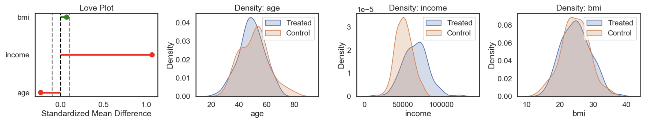
Regression adjustment after matching (RAAM)
To mitigate residual imbalance bias, it’s common to fit a regression model on the matched sample to adjust for any remaining differences in covariates. After matching, you construct a dataset containing all treated units and their matched controls. This can be structured in a stacked format like below:
| unit_id | matched_set_id | treatment | X₁ | X₂ | outcome |
|---|---|---|---|---|---|
| 101 | 1 | 1 | … | … | … |
| 205 | 1 | 0 | … | … | … |
| 309 | 1 | 0 | … | … | … |
| 102 | 2 | 1 | … | … | … |
| 220 | 2 | 0 | … | … | … |
Some control units may appear in multiple matched sets if matching is performed with replacement. Rather than duplicating these units, you can assign weights based on how many times each unit appears across sets. Now we have a more homogeneous sample, with smaller differences between treated and control units. We then fit a regression model to estimate the treatment effect while adjusting for remaining differences in covariates:
\[Y_i = \alpha + \tau T_i + \sum_{k=1}^p \beta_k X_{ki} + \epsilon_i\]Where:
- \(Y_i\) is the outcome for unit \(i\),
- \(T_i\) is the treatment indicator (\(1\) if treated, \(0\) otherwise),
- \(X_{ki}\) are the covariates for unit \(i\),
- \(\alpha\) is the intercept,
- \(\tau\) is the coefficient estimating the treatment effect,
- \(\beta_k\) are coefficients for covariates,
- \(\epsilon_i\) is the error term.
The regression model does not use the matched set IDs directly. Matching restricts the sample to comparable units, and regression adjusts for any small differences that remain. Conceptually, the regression projects units onto their expected outcomes given covariates, then estimates the average difference between treated and control units on that adjusted scale. Because some units may be reused, standard errors should be corrected. You can either: use robust standard errors clustered on matched set ID, or apply bootstrapping (repeat matching and regression on resampled data).
This hybrid approach leverages the strengths of both methods:
- Matching is non-parametric, imposing fewer assumptions about the relationship between covariates and outcome, making it robust to model misspecification.
- Regression is applied locally on matched pairs, fine-tuning the estimate without extrapolating beyond comparable units.
To get the ATE via reweighting we need to perform bidirectional matching (match treated units to controls and control units to treated units). To combine this with regression adjustment, you can either:
- Fit separate regressions on the matched treated and matched control samples, and average the treatment effects; or,
- Combine the matched samples into one dataset and fit a single regression, using weights to account for reuse and group size.
As always, careful selection of confounders and balance diagnostics are crucial for reliable causal inference.
Causal strength
Matching helps reduce bias by creating comparable groups (approximating a randomised experiment), but it relies on strong assumptions:
-
Exchangeability (No unmeasured confounding): Matching can only balance observed covariates. If important confounders are not measured or not included in the matching process, estimates will remain biased. Further, matching reduces differences but doesn’t guarantee perfect balance (residual bias). Any remaining imbalance can bias effect estimates, especially if not adjusted for (e.g. with regression).
-
Positivity (Overlap): If treated and control units differ too much on covariates, good matches cannot be found. Matching either forces poor matches (increasing bias) or discards unmatched units (increasing variance).
-
Consistency (Well-defined treatment): Matching assumes that the treatment is consistently defined across units. In observational settings, treatment might vary in form, intensity, or timing. If treatment meaning varies across matched pairs, the estimated effect may not correspond to a single well-defined intervention.
Propensity score methods
Propensity score methods also reduce confounding by balancing covariates between treated and untreated groups. However, instead of directly adjusting for all confounders \(X\), we estimate a single balancing score:
\[e(X) = \mathbb{P}(T = 1 \mid X)\]This is the probability of receiving treatment given covariates. If treatment assignment depends on \(X\), then individuals with different \(X\) values may have different chances of being treated. But if \(X\) includes all confounders, then treatment is conditionally independent of the potential outcomes:
\[(Y(0), Y(1)) \perp T \mid X\]Rosenbaum and Rubin (1983) showed that this implies:
\[(Y(0), Y(1)) \perp T \mid e(X)\]So instead of adjusting for high-dimensional \(X\), we can adjust for the scalar \(e(X)\) and it will work in the same way. This simplifies matching, stratification, or weighting methods as individuals with similar propensity scores can be treated as if randomly assigned, even if their raw covariates differ. In effect, the propensity score compresses all relevant confounding information from \(X\) into a single variable.
Estimating $e(X)$
Since the treatment assignment mechanism is unknown in observational data, we estimate the propensity score $e(X)$ using a predictive model. Typically this would be logistic regression for binary treatments. More flexible models like random forests or gradient boosting can also be used. But the goal isn’t high predictive accuracy; it’s covariate balance. A model that includes variables highly predictive of treatment but unrelated to the outcome (i.e. not confounders) may boost predictive accuracy but worsen precision by increasing variance in the ATE estimate. For example, suppose you’re estimating the effect of a training program on productivity. You fit two models:
- Model A uses just the true confounders (age and experience), and achieves 70% accuracy.
- Model B adds irrelevant but predictive variables, like office location and day of week, and achieves 90% accuracy.
Despite the higher accuracy, Model B may yield worse balance on the confounders, causing biased causal estimates. That’s because the model is optimizing for prediction, allowing irrelevant variables to dominate instead of balancing the confounders.
Checking positivity
It’s important that treated and untreated units overlap. That is, everyone must have some chance of receiving and not receiving treatment: \(0 < e(X) < 1\). This is known as the positivity assumption. You can check this by comparing the distributions of propensity scores in the treated and untreated groups. Ideally, they should substantially overlap across the full range, and be smooth, with no scores close to 0 or 1. Propensity scores near 0 or 1 mean someone is almost guaranteed to be treated (or not), which causes estimators like the inverse probability weight to blow up, increasing the variance of the ATE (makes it sensitive to a few influential observations). As a rule of thumb, no individual should get a weight over 20. Some will trim the propensity scores to limit the range (e.g. 0.05 to 0.95), but this can introduce bias. Another option is to trim observations outside the overlap region (i.e. drop treated with no comparable untreated match), but this limits the generalisability.
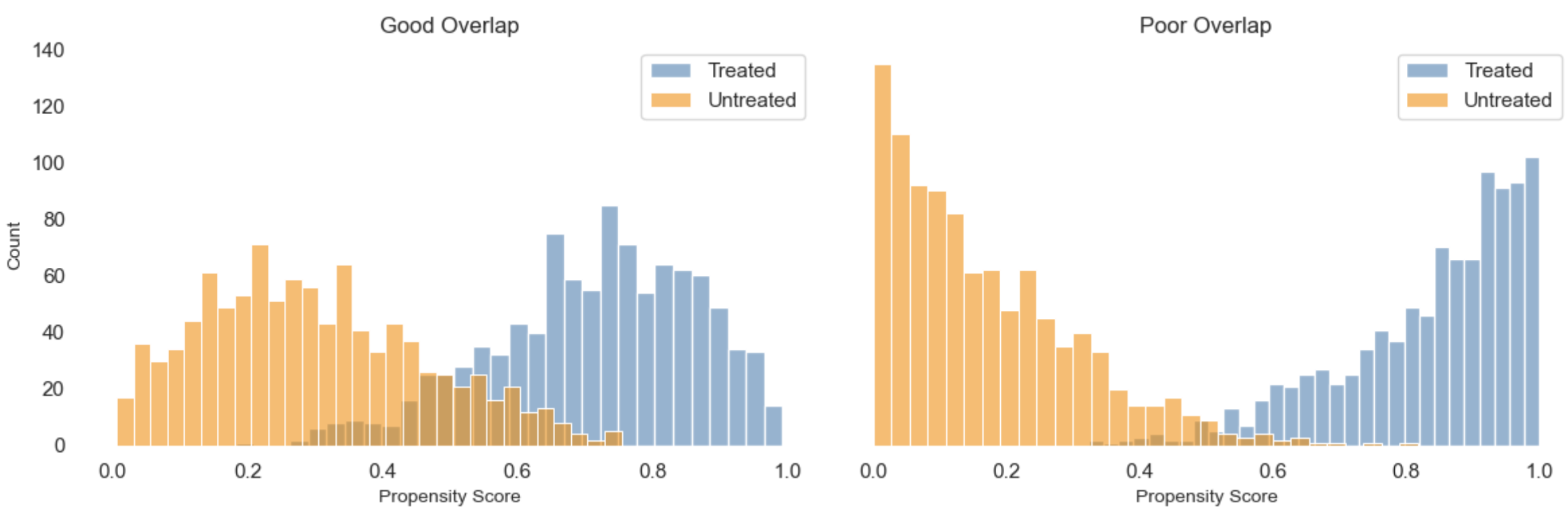
Propensity scores + matching
Propensity scores offer a solution to the curse of dimensionality in matching. Instead of matching on all covariates directly, we match on a single summary score: the propensity score. This reduces the dimensionality of the problem and ensures that units are matched based on their likelihood of receiving treatment. In this way it focuses the comparison on units that are similar in terms of confounding risk.
As discussed in the matching section, a caliper can be set to control the maximum allowable difference in propensity scores for a pair to be matched (e.g. 0.2 standard deviations). However, there are some important caveats:
- Overlap is still essential: If treated and control units do not share common support (for example, if their propensity scores are close to 0 or 1), good matches may not exist. This can lead to biased estimates.
- Bias-variance trade-off: Tight matching using small calipers can reduce bias by ensuring closer matches, but it also increases variance because fewer units are retained. Looser calipers allow more matches and reduce variance, but at the risk of introducing bias through poor matches.
- Standard errors require care: The propensity score is estimated, not observed. Standard error calculations that ignore this will understate the true uncertainty. Adjustments or bootstrapping methods are typically needed.
Matching is intuitive and transparent. However, it depends entirely on the quality of the propensity score model. If the model is misspecified, the resulting matches can still be unbalanced, and bias will remain.
Using e(X) as a weight
The estimated propensity score can also be used as a weight to construct a pseudo-population where treatment assignment is independent of observed covariates. In the next sections, we’ll walk through three widely used weighting-based approaches:
| Method | What it does (in plain terms) | Efficiency & Robustness | When to use it (and what to watch out for) |
|---|---|---|---|
| IPW | Reweights observations by how unlikely their treatment was, based on covariates. | Low efficiency; sensitive to extreme weights; not robust to misspecification. | Use when the treatment model is well understood and overlap is strong. May require trimming or weight stabilization. |
| AIPW | Combines outcome predictions with IPW to reduce bias if either model is wrong. | Moderately efficient; doubly robust; variance can be high without cross-fitting. | Useful when you want extra protection against misspecification. Works well with flexible outcome models, but cross-fitting is important to avoid overfitting. |
| TMLE | Starts with an outcome model, then “nudges” it using the treatment model to improve accuracy. | Most efficient; doubly robust; targeting step improves finite-sample performance. | Preferred when using ML models and valid inference is important. Requires careful implementation (e.g. cross-fitting) but yields strong theoretical guarantees. |
1) Inverse Probability Weighting (IPW)
Inverse Probability Weighting (IPW) leverages the propensity score $e(X)$ to reweight each unit’s outcome, effectively creating a synthetic population where treatment assignment is independent of $X$ (i.e. adjusting for confounding). The weight is inversely proportional to their probability of receiving their observed treatment. Specifically:
- Treated units are weighted by $\frac{1}{e(X)}$, so individuals who were unlikely to be treated but received treatment have greater influence.
- Control units are weighted by $\frac{1}{1 - e(X)}$, giving more weight to those unlikely to be untreated but actually untreated.
In this way it gives more influence to people who are “underrepresented” in their group: those treated despite low probability, or untreated despite high probability. We’re creating two comparable synthetic populations here (each the same size as the original), one where everyone is treated and one where no one is. Comparing them then gives us the conditional mean difference using only \(e(X)\) instead of the full set of covariates.
Recall the conditional mean difference (difference in outcomes between the treated and untreated):
\[\mathbb{E}[Y \mid X, T = 1] - \mathbb{E}[Y \mid X, T = 0]\]Re-writing this using the propensity scores, the left hand side becomes:
\[\mathbb{E}\left[ \left. \frac{Y}{e(x)} \,\right|\, X, T = 1 \right] P(T)\]We take the outcomes of treated people, reweight them using the inverse of their treatment probability (\(\frac{Y}{e(x)}\)). This downweights those with a high chance of treatment and upweights those with a low chance so we don’t over-represent those who were likely to be treated. This is then scaled by how common treatment is overall to give us an estimate of what everyone would have experienced, had they all received the treatment.
Then the right hand side follows the same idea for the untreated:
\[\mathbb{E}\left[ \left. \frac{Y}{1 - e(x)} \,\right|\, X, T = 0 \right] (1 - P(T))\]This uses \(1-e(x)\) in the denominator (the probability of not being treated, given X), so \(\frac{Y}{1-e(x)}\) gives more weight to those unlikely to be untreated (but were). Scaling by how common it is to be untreated (1-P(T)), this estimates what the entire population would have experienced if no one had received the treatment, by appropriately reweighting the observed outcomes of untreated individuals.
Putting these together and simplifying, the expected potential outcomes under treatment and control are estimated as:
\[\mathbb{E}\left[ \frac{T \cdot Y}{e(X)} \right] \quad \text{and} \quad \mathbb{E}\left[ \frac{(1 - T) \cdot Y}{1 - e(X)} \right]\]Subtracting these gives an estimate of the Average Treatment Effect (ATE):
\[\mathbb{E}\left[ \frac{T \cdot Y}{e(X)} - \frac{(1 - T) \cdot Y}{1 - e(X)} \right]\]This can also be written more compactly as:
\[\mathbb{E} \left[ Y \cdot \frac{T - e(X)}{e(X)(1 - e(X))} \right]\]Given the propensity score is an estimation, we need to account for this in the standard error of the ATE (e.g. by bootstrapping an ATE sampling distribution).
2) Augmented Inverse Probability Weighting (AIPW)
Propensity scores can also be combined with an outcome model (e.g. regression) to produce a doubly robust estimator. The key advantage is that you get a consistent estimate of the average treatment effect (ATE) if either the outcome model or the propensity score model is correctly specified. Since both methods alone have weaknesses (outcome models can be biased, and propensity score weighting can be unstable), combining them lets one “lean on” the other when it is misspecified.
For example, consider the Augmented Inverse Probability Weighting (AIPW) estimator:
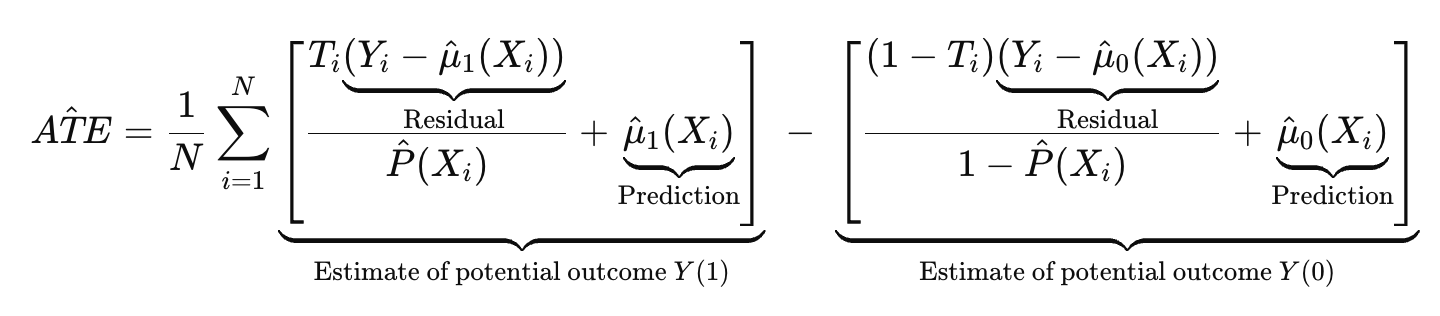
Where:
- \(T_i\) is the treatment assignment (1=treated)
- \(\hat{\mu}_1(X) = \mathbb{E}[Y \mid X, T = 1]\) is the predicted outcome from the outcome model for the treated (trained on T=1 only)
- \(\hat{\mu}_0(X) = \mathbb{E}[Y \mid X, T = 0]\) is the predicted outcome from the outcome model for the untreated (trained on T=0 only)
- \(\hat{P}(X) = \mathbb{P}(T = 1 \mid X)\) is the propensity score model (trained on all)
Note that AIPW can use either separate outcome models for treated and untreated groups or a single joint model with treatment as an input. Typically, two separate models are preferred when treatment effect heterogeneity is suspected or when there is sufficient data in both groups to flexibly model outcomes. A single joint model is often used when sample size is limited or when the treatment effect is believed to modify the outcome additively or smoothly across covariates. While simpler models are generally preferred for the propensity score to avoid instability, flexible machine learning models can be used for the outcome model to better capture complex and nonlinear relationships. Although double robustness provides some protection against misspecification, cross-fitting is recommended to reduce overfitting. This involves splitting the data into folds and evaluating each fold using models trained on the other folds, which helps preserve the theoretical guarantees of AIPW.
The key idea is to create two synthetic populations to estimate potential outcomes: one where everyone is treated (to estimate $Y(1)$) and one where everyone is untreated (to estimate $Y(0)$). Like standardisation, AIPW uses an outcome model to provide baseline predictions $\hat{\mu}_1(X), \hat{\mu}_0(X)$. But AIPW goes further by incorporating a correction based on the treatment assignment model. Specifically, the residuals (observed outcome minus predicted outcome) are weighted by the inverse of the propensity score for the observed treatment. This gives more influence to residuals from units with unlikely treatment assignments; typically the regions where the outcome model is more likely to be biased. For units not observed in a treatment group, the weighted residual is zero, so their contribution relies solely on the model prediction, as in standardisation. By combining outcome regression with inverse probability weighting, AIPW reduces bias from model misspecification and remains consistent if either model is correct. Because the variance reflects uncertainty from both models and residual noise, bootstrapping is typically the simplest and most robust way to compute standard errors.
Example
Imagine we want to estimate the effect of a promotion on spending for all users, but income (an important confounder), is imperfectly measured. High-income customers in our data were more likely to get the promotion and tend to spend more, so a naive regression may overestimate the promotion effect. If some customer types are rarely treated, outcome predictions there may be poor. By weighting the residuals inversely by the probability of receiving treatment, we “rescale” these residuals to reflect the overall population better, providing a correction in underrepresented regions. The residual tells us how wrong the outcome model was, and the weighting ensures this correction is applied in proportion to where the model is likely to be wrong (i.e. in underrepresented areas).
- If the outcome model is good: the residuals are small, so the correction term adds little, and the estimate relies on the correct outcome model predictions (i.e. it doesn’t matter if the propensity scores are wrong).
- If the outcome model is poor: the residuals are large, and the correction (weighted by the correctly specified propensity score) helps adjust bias, making the estimator rely more on propensity weighting. Assuming the propensity model is correct (i.e. \(\mathbb{E}\big[ T_i - \hat{P}(X_i) \big] = 0\)), it reduces down to an IPW estimator (\(\frac{T_i Y_i}{\hat{P}(X_i)}\)).
This means we have two chances to get unbiased estimates: either the outcome model is correct, or the propensity score model is correct.
3) Targeted Maximum Likelihood Estimation (TMLE)
TMLE builds on AIPW, using the same inputs but a different method for combining models to improve efficiency, especially in finite samples. While AIPW plugs in the model estimates directly into a closed-form expression, TMLE takes an extra step to update the outcome model using a likelihood-based adjustment. This makes TMLE particularly useful when using flexible machine learning models, such as random forests or gradient boosting, while still retaining statistical guarantees like valid confidence intervals.
| TMLE starts from the insight that both outcome models (predicting E[Y | T, X]) and treatment models (estimating P(T | X)) can be error-prone, especially when estimated with flexible algorithms. TMLE reduces these errors by targeting the initial outcome estimate using information from the treatment model. The result is a final estimator with desirable properties like consistency, efficiency, and double robustness. |
At a high level, TMLE proceeds as follows:
Estimate the outcome model
Use any supervised learning method to estimate the expected outcome as a function of treatment and covariates:
\[\hat{Q}(T, X) \approx \mathbb{E}[Y \mid T, X]\]This could be linear regression, random forests, gradient boosting, or any other reasonable predictor. The goal is a good initial estimate of expected outcomes.
Estimate the treatment model (propensity score)
Estimate the conditional probability of receiving treatment T given covariates X:
\[\hat{g}(T \mid X)\]For binary treatment, this is the usual propensity score. For continuous or multi-valued treatments, more complex models are needed to estimate the treatment assignment mechanism.
Compute the clever covariate
The clever covariate captures how much each observation contributes to the correction. For binary treatment, it is typically:
\[H(T, X) = \frac{I(T = 1)}{\hat{g}(1 \mid X)} - \frac{I(T = 0)}{\hat{g}(0 \mid X)}\]This covariate encodes both the direction and size of the adjustment needed to address confounding.
Update the outcome model
The initial outcome model $\hat{Q}$ is updated through a targeted maximum likelihood step. This involves solving a likelihood-based estimating equation that incorporates the clever covariate, effectively nudging $\hat{Q}$ so that it better respects the observed treatment mechanism. In practice, this targeting step often involves fitting a small regression (for example, logistic or linear) using the clever covariate as a feature and the initial predicted outcomes as offsets.
This targeting step ensures that the final estimator is consistent if either the outcome model or the treatment model is correct, and efficient when both are correct. This is the double robustness property.
Estimate the treatment effect
Once the updated outcome model $\hat{Q}^*$ is obtained, potential outcomes under treatment and control are estimated:
\[\hat{\mu}_1 = \frac{1}{n} \sum_{i=1}^n \hat{Q}^*(1, X_i), \quad \hat{\mu}_0 = \frac{1}{n} \sum_{i=1}^n \hat{Q}^*(0, X_i)\]Then the average treatment effect (ATE) is computed as:
\[\widehat{\text{ATE}} = \hat{\mu}_1 - \hat{\mu}_0\]TMLE combines outcome and treatment modeling in a way that protects against misspecification in either one. Like AIPW, it is doubly robust: consistent if at least one of the models is correctly specified. In addition, the targeting step improves efficiency by reducing bias in the initial outcome predictions using information from the treatment model. To ensure valid inference when using flexible learners, TMLE typically includes cross-fitting. The data is split into folds, and each fold is evaluated using models trained on the others. This reduces overfitting and preserves the theoretical guarantees of TMLE, even with high-capacity models.
Diagnostics: Checking Covariate Balance
Regardless of the method chosen from above, it is essential to check whether the treatment and control groups are balanced on key covariates to draw valid causal conclusions. This means their distributions should be similar enough that comparisons approximate a randomized experiment.
With weighting methods (IPW, AIPW, TMLE), balance is assessed in the weighted sample: each observation is reweighted by the inverse of its estimated propensity score, and the resulting covariate distributions are compared across groups. With matching, balance is evaluated in the matched sample, which includes only treated and control units that were successfully paired. If variable-ratio or replacement matching is used, match weights should be incorporated into diagnostics.
Typical balance diagnostics include:
- Standardized mean differences (SMDs) for each covariate. Aim for an absolute SMD below 0.1.
- Variance ratios comparing the spread of each covariate between groups. A common threshold is between 0.8 and 1.25.
- Visualizations such as density plots, empirical CDFs, or love plots to compare covariate distributions before and after adjustment.
Diagnostics should be performed both before and after adjustment to assess how much imbalance remains. If balance is still poor, consider the following:
- Revising the propensity score model. Include interaction terms, nonlinear features, or additional confounders.
- Trimming or restricting to common support. Remove observations with extreme propensity scores or limited overlap between groups.
- Switching to a different adjustment method. If IPW leads to extreme weights or matching performs poorly, outcome modeling or hybrid methods like AIPW or TMLE may be more appropriate.
- Re-evaluating the study design. Persistent imbalance may indicate misspecification of the treatment mechanism or missing confounders.
In short, covariate balance diagnostics are a necessary part of any causal analysis. They tell you whether your adjustment method has sufficiently addressed observed confounding. If balance is poor, the resulting estimates may still be biased, and further refinement or design changes may be needed.
Causal Strength
Propensity score methods provide a useful framework for estimating causal effects when confounding is strong and high-dimensional, but fully observed. Methods like IPW, AIPW, TMLE, and matching differ in how they adjust for confounding, but all rely on the same core assumptions. Correct model specification and the Stable Unit Treatment Value Assumption (SUTVA) are required for all, but the reliability of results ultimately depends on the validity of the following identifiability conditions:
-
Exchangeability (no unmeasured confounding): Given observed covariates $X$, treatment assignment is independent of potential outcomes. This means treatment is as good as randomly assigned after adjusting for $X$. If important confounders are missing, estimates can be biased due to omitted variable bias. Because this assumption cannot be tested directly, it must be justified based on subject-matter knowledge and study design.
-
Positivity (overlap): Each individual must have a positive probability of receiving both treatment and control. That is, the estimated propensity score should be strictly between 0 and 1. When certain groups always or never receive treatment, comparisons become unreliable. Limited overlap can result in extreme weights and unstable estimates, especially in weighting methods. In such cases, trimming or restricting to regions with good overlap may help, though this can limit generalizability.
-
Consistency: The treatment must be clearly defined and applied uniformly. Each individual’s observed outcome under their actual treatment corresponds to their potential outcome for that treatment. Inconsistent or poorly defined treatments can violate this assumption.
Causal inference using propensity scores requires more than just applying a method. It depends on careful diagnostics, transparent assumptions, and a willingness to revise the model or approach if balance cannot be achieved. When these elements are in place, propensity score methods can provide credible estimates of causal effects from observational data.
Generalized Propensity Score (GPS)
Most common propensity score methods are designed for binary treatments and do not naturally extend to continuous treatments without modification. The Generalized Propensity Score (GPS) extends the concept to continuous treatments (such as dosage levels) by modeling the conditional density of the treatment given covariates:
\[r(t, X) = f_{T|X}(t | X)\]Unlike the binary propensity score, which gives a scalar probability of treatment assignment, the GPS is a continuous function: it describes the conditional probability density of receiving a particular treatment level given covariates. In other words, it tells us how likely an observation is to receive a particular treatment level based on its characteristics.
| Specifically, for a continuous treatment T, the GPS at level t and covariates X is defined as the conditional density $r(t, X) = f_{T | X}(t \mid X)$. In practice, the GPS is often estimated using a parametric model for $T \mid X$, most commonly assuming a normal distribution. For example: |
-
Fit a linear regression model to estimate expected treatment: Regress the treatment variable T on covariates X:
\[T = X^\top \beta + \varepsilon, \quad \varepsilon \sim \mathcal{N}(0, \sigma^2)\] -
Estimate parameters: From the fitted model, obtain estimates $\hat{\beta}$ and the residual variance $\hat{\sigma}^2$. Not everyone receives exactly the predicted treatment. This variation reflects randomness, measurement error, or unobserved factors, and is used to construct the conditional treatment density.
-
Compute the conditional mean: For each observation i, compute the predicted treatment level based on its covariates:
\[\hat{\mu}_i = X_i^\top \hat{\beta}\] -
Evaluate the conditional density (GPS): We ask how likely the observed treatment level $t_i$ is, given the predicted value $\hat{\mu}_i$. The estimated GPS is the value of the normal density at the observed treatment:
\[\hat{r}(t_i, X_i) = \frac{1}{\sqrt{2\pi\hat{\sigma}^2}} \exp\left( -\frac{(t_i - \hat{\mu}_i)^2}{2\hat{\sigma}^2} \right)\]
Non-parametric alternatives such as kernel density estimation or Gaussian processes can be used when the normality assumption is not appropriate.
Once estimated, the GPS serves as a balancing score. Just like the binary propensity score, the idea is that conditional on the GPS, the covariates X are independent of treatment T. This mimics a randomized design and allows us to isolate the effect of treatment intensity. The GPS can then be used in different causal estimation methods:
- Regression adjustment: Model the outcome as a function of treatment and GPS, $\mathbb{E}[Y \mid T = t, r(t, X)]$, then average across the covariate distribution to get $\mu(t)$, the dose-response curve.
- Stratification: Discretize the treatment and GPS into intervals. Estimate average outcomes within each stratum, then aggregate across strata.
- Matching: Match units with similar GPS values at the same or similar treatment levels to create localized comparisons that approximate a randomized experiment.
To estimate a causal effect such as the average treatment effect between two treatment levels $t_1$ and $t_2$, compute $\mu(t_2) - \mu(t_1)$ from the estimated dose-response curve.
Diagnostics
Diagnostics for GPS methods play the same role as in binary propensity score methods: checking for covariate balance and ensuring sufficient overlap. However, the continuous treatment adds complexity.
-
Covariate balance checks: As in the binary case, we check that units with similar GPS values are comparable in terms of their covariates. For continuous treatments, this usually means assessing covariate balance within strata defined by both treatment level and GPS. Methods include:
- Standardized mean differences within narrow bands of treatment and GPS.
- Stratified plots comparing covariate distributions across treatment intensities.
-
Common support and overlap: Just as in the binary case, we need sufficient overlap in the GPS distribution across treatment levels. This is often visualized by plotting GPS density across treatment values or examining the joint distribution of treatment and GPS. Lack of overlap suggests that causal effects may not be reliably identified in some regions of treatment space.
-
Model fit diagnostics: If the GPS is estimated using a parametric model like linear regression with Gaussian residuals, model assumptions should be checked. This includes residual plots, QQ-plots, and considering more flexible models (e.g. splines or non-parametric estimators) if needed.
Causal strength
GPS methods rely on extensions of the standard assumptions for causal inference:
-
Weak unconfoundedness: The potential outcome at each treatment level t is independent of treatment assignment, given covariates X:
\[Y(t) \perp\!\!\!\perp T \mid X \quad \text{for all } t\] -
Overlap: Every unit must have positive probability density of receiving treatment at the levels of interest:
\[f_{T|X}(t \mid X) > 0\]
GPS provides a principled way to recover full dose-response relationships without reducing treatment to binary form. But it can be sensitive to model misspecification and issues with support. Diagnostics such as GPS balance checks and overlap plots are essential to validate assumptions and ensure credible inference.
Orthogonal Machine Learning (Double ML)
Orthogonal Machine Learning (OML) is a method specifically designed to estimate causal effects using flexible machine learning models, while guarding against overfitting and bias from high-dimensional or complex covariates. While ML models can capture complex relationships, they don’t necessarily focus on estimating the treatment effect. So called “nuisance” variables, which influence both the treatment and outcome but are not of primary interest, can absorb part of the treatment effect. This leads to a biased coefficient estimate. OML addresses this by separating (orthogonalizing) the variation in treatment and outcome that is explained by covariates, allowing the causal effect to be estimated from the residual variation that remains. While the nuisance models use ML, the final step estimates the treatment effect using a simple parametric model, typically a linear regression on these residuals. This means it assumes the causal effect is well approximated by a linear or similarly simple function after confounding has been removed. Therefore, it still depends on correct specification of the final treatment effect model to yield unbiased causal estimates.
Orthogonalization
The fundamental idea is to decompose both the treatment and the outcome into components that are orthogonal, or uncorrelated, with respect to the nuisance variables. To do this, first we fit flexible ML models to predict the treatment and outcome using the nuisance variables. Using the residuals of those models (to remove the effect of the nuisance variables), we then fit a simple regression to isolate the effect of the treatment on the outcome:
-
Predict Treatment: Fit an ML model \(M_t(X)\) to predict the treatment \(T\) from the covariates \(X\) (like a propensity score model). The residuals \(\tilde{t} = T - M_t(X)\) represent the portion of \(T\) that is unrelated to \(X\).
-
Predict Outcome: Fit an ML model \(M_y(X)\) to predict the outcome \(Y\) from \(X\). The residuals \(\tilde{y} = Y - M_y(X)\) represent the portion of \(Y\) that is unrelated to \(X\).
-
Estimate the Treatment Effect: The causal effect $\theta$ is then estimated by regressing \(\tilde{y}\) on \(\tilde{t}\), ensuring that the estimated effect reflects the part of \(Y\) that is attributable to \(T\) after adjusting for \(X\).
$\tilde{y}_i = \alpha + \theta \tilde{t}_i + \varepsilon_i$
A key strength of this approach is that small errors in estimating the nuisance parameters do not bias the estimated treatment effect, provided those errors are orthogonal to the treatment residuals. However, there is a risk of the ML models over-fitting, and then the regression underestimating the treatment effect.
Cross-fitting
To avoid overfitting and to ensure valid confidence intervals, it is recommended to use cross-fitting. This involves training the nuisance models on one subset of the data and computing residuals on a separate subset.Specifically, the data is split into $K$ folds. For each fold $k$, you:
- Train the treatment $M_t(X)$ and outcome $M_y(X)$ models on the other $K-1$ folds (excluding fold $k$),
- Use those models to compute the residuals $\tilde{t}_i = T_i - M_t(X_i)$ and $\tilde{y}_i = Y_i - M_y(X_i)only on fold $k$.
Each residual is computed using models that didn’t see that observation (out-of-fold), reducing bias from overfitting. After processing all folds, you concatenate the residuals $\tilde{t}_i$ and $\tilde{y}_i$ to create the full-length vectors of orthogonalized treatment and outcome. Then you can estimate the treatment effect as before by regressing \(\tilde{y}\) on \(\tilde{t}\).
Benefits
In outcome regression, we get more precise estimates as we collect more data. Specifically, our estimation error shrinks at a rate of $1/\sqrt{n}$, called root-$n$ consistency. This means that as the sample size $n$ grows, our parameter estimates converge quickly to the true value, and the distribution of the estimator becomes approximately normal. This is what enables us to construct valid confidence intervals and perform reliable hypothesis tests.
Standard ML models generally converge more slowly. They prioritize prediction accuracy over statistical inference. For example, they often introduce bias to reduce variance (e.g. via regularization, tree pruning, or early stopping), which improves out-of-sample prediction performance. Their goal is to minimize a loss function, not to estimate interpretable parameters, so there’s no guarantee their coefficients (if they have any) are unbiased, consistent, or asymptotically normal. In high-dimensional settings, ML models may need exponentially more data to learn the underlying function accurately. This slows convergence further and makes it harder to quantify uncertainty. As a result, confidence intervals and hypothesis tests based directly on standard ML models are often invalid or unavailable.
The great thing about OML with cross-fitting is that it can achieve root-$n$ consistency, enabling reliable and statistically valid estimates (including valid confidence intervals and hypothesis tests), even when using complex machine learning models and high-dimensional covariates.
-
Orthogonalization removes the influence of high-dimensional nuisance variables by residualizing both the treatment and the outcome using flexible ML models. The final estimate is obtained by regressing the outcome residuals on the treatment residuals, isolating the variation in treatment that is independent of confounders. This setup ensures that small errors in the nuisance models (common when using machine learning), do not bias the treatment effect estimate, provided these errors are orthogonal (i.e. uncorrelated) to the residualized treatment.
-
Cross-fitting strengthens this robustness, preventinh overfitting and ensuring that the residuals used in the final regression are independent of the models that generated them. Crucially, this separation allows the final treatment effect estimator to behave like a classical estimator, with known asymptotic properties. Meaning it enables the use of standard formulas to construct valid confidence intervals and perform hypothesis testing, even in high-dimensional or flexible ML settings.
Causal strength
Orthogonal Machine Learning extends the familiar idea of adjusting for covariates in outcome regression to more flexible settings with machine learning models. When dealing with high-dimensional or complex confounding it can reduce bias, assuming the first-stage models approximate the true relationships well (no substantial misspecification). Cross-fitting reduces the risk of overfitting and bias, but poor first-stage performance can still affect precision. Importantly, the reliability of OML still rests on the same core identification assumptions as the other observational methods:
-
Exchangeability (no unmeasured confounding): Conditional on the observed covariates $X$, treatment assignment is assumed to be as good as random. OML can flexibly adjust for complex confounding patterns, but cannot recover from omitted variables that affect both treatment and outcome. As with other methods, this assumption is untestable and must be justified by domain knowledge and thoughtful covariate selection.
-
Positivity (overlap): For OML to work well, there must be sufficient overlap between treated and untreated units across the covariate space. If some units are deterministically treated or untreated based on $X$, residualizing the treatment won’t eliminate extrapolation bias. Trimming or restricting the analysis to areas of common support may still be necessary.
-
Consistency: The treatment must be clearly defined and uniformly applied across observations. If the treatment varies in how it’s implemented or is mismeasured, the causal interpretation of the estimated effect becomes unclear.
Orthogonalization improves robustness to errors in nuisance estimation, but it does not remove the need for thoughtful variable selection, strong overlap, or the absence of unmeasured confounding. As always, careful diagnostics, sensitivity analyses, and an understanding of the data-generating process are essential to ensure valid causal inference.
Adjustment methods comparison
To recap, adjustment-based methods estimate causal effects by controlling for confounding variables in observed data. However, they differ in how they construct comparability between treated and control groups: some model outcomes directly, some weight or match observations, and others combine strategies for robustness. Each has it’s strengths and weaknesses to consider:
| Method | How It Works | Key Strengths | Key Limitations |
|---|---|---|---|
| Outcome Regression | Fits a model for $\mathbb{E}[Y \mid T, X]$ using the full dataset, then predicts outcomes under treatment and control for each unit and averages the difference to estimate ATE. Preferable when overlap is strong and the outcome model is correctly specified or can be well approximated. | Uses all data; flexible modeling of outcomes; direct estimate of conditional effects. | Sensitive to misspecification of outcome model; extrapolation risk in poor overlap regions. |
| G-computation (standardisation / g-formula) | Predicts potential outcomes for all units under each treatment level and averages over the covariate distribution to get the marginal ATE. Preferable when flexible outcome modeling is feasible and marginal effects are the focus. | Intuitive population-level estimate; uses entire sample. | Shares regression’s sensitivity to model misspecification; no explicit confounding adjustment via treatment modeling. |
| Matching (on covariates or PS) | Creates matched pairs or sets of treated and control units based on similarity, and estimates ATE from these matched samples. Preferable when overlap is limited and prioritizing local comparability for valid ATE. | Avoids extrapolation; emphasizes direct comparability; less model-dependent. | Reduces sample size; may increase variance; excludes unmatched units. |
| IPW | Weights units by the inverse probability of their received treatment, creating a synthetic balanced sample; estimates ATE from weighted averages. Preferable when overlap is sufficient and the propensity score model is well specified and calibrated. | Model-free outcome estimation; consistent if propensity model is correct; conceptually straightforward. | Can produce unstable estimates with extreme weights from poor overlap. |
| AIPW (Doubly Robust) | Combines outcome regression and IPW to estimate ATE; remains consistent if either the outcome or propensity model is correct. Preferable when using flexible outcome and treatment models and robustness is important. | Double robustness reduces bias; more stable than IPW alone; suitable with flexible models. | Still sensitive to extreme weights; cross-fitting recommended with machine learning. |
| TMLE (Targeted MLE) | Starts with an initial outcome model, then uses the propensity score to “target” or update it, refining the ATE estimate for efficiency and valid inference. Preferable when using machine learning and seeking efficient, statistically rigorous ATE estimates. | Double robust with improved finite-sample properties; compatible with ML; provides valid confidence intervals. | More complex implementation; cross-fitting required for reliable inference. |
| Generalized Propensity Score (GPS) | Extends propensity scores to continuous or multi-valued treatments; estimates dose-response curves or marginal ATE accordingly. Preferable when treatments are continuous or multi-level, and dose-response or marginal effects are needed. | Enables causal inference beyond binary treatments; estimates marginal effects. | Requires strong assumptions and precise treatment density modeling. |
| OML (Orthogonal ML) | Uses orthogonal moments and cross-fitting to debias machine learning–based ATE estimators, especially in high-dimensional covariate spaces. Preferable for high-dimensional settings with complex outcome and treatment relationships modeled flexibly. | Provides valid inference with complex ML; handles high-dimensional data; robust to overfitting. | More abstract and technically involved; requires careful tuning and validation. |
To give a specific example, let’s think about how the different methods would handle sparse or imbalanced subgroups (where there are few treated or control observations, so nearly violating positivity):
- Outcome regression models extrapolate across all subgroups by relying on the specified functional form to predict outcomes even where treatment variation is minimal. This means it uses information from other parts of the covariate space to estimate effects in underrepresented groups, which can lead to bias if the model is misspecified or the extrapolation is unwarranted.
- Matching implicitly trims or excludes units in sparse subgroups that do not have suitable counterparts. If treated units lack similar controls (or vice versa), those units are discarded or downweighted, which avoids extrapolation but can reduce sample size and increase variance. This approach prioritizes local comparability and avoids relying on untested assumptions in poorly represented regions.
- Inverse probability weighting (IPW) reweights observations to create a synthetic sample balanced across treatment groups. However, in sparse or imbalanced subgroups, propensity scores can be extreme (near 0 or 1), causing large weights that increase variance and make estimates unstable. Without additional adjustments, IPW can be sensitive to poor overlap.
- Robust methods like Augmented IPW (AIPW), Targeted Maximum Likelihood Estimation (TMLE), and Orthogonal Machine Learning (OML) combine the strengths of both modeling and weighting. They flexibly adjust for confounding by leveraging both outcome models and propensity scores. This allows them to reduce bias from misspecification or poor overlap while controlling variance through techniques like cross-fitting and targeting. These methods avoid the extremes of pure extrapolation or outright trimming by balancing the trade-off between bias and variance, resulting in more reliable estimates in challenging data scenarios.
This is an example where you might favor robust methods like AIPW or TMLE, especially when you have complex relationships and some risk of model misspecification, but also want to mitigate issues caused by limited overlap or sparse data regions.
Quasi-Experimental Designs
Now we’re moving on to quasi-experimental designs. The adjustment-based methods discussed earlier (e.g. regression, matching, propensity scores, OML) require that all relevant confounders are observed and correctly included in the model; an assumption that is often violated in practice. Quasi-experimental designs address this limitation by leveraging natural experiments, study design features, or structural breaks that introduce variation in treatment assignment for reasons unrelated to potential outcomes. This can make their identifying assumptions more plausible, but also limits their scope and generalisability.
Common quasi-experimental methods include:
- Instrumental Variable (IV) analysis: Uses external variation that influences treatment but not directly the outcome to handle unmeasured confounding.
- Difference-in-Differences (DiD): Compares changes over time between treated and control groups in panel data (multiple units over time).
- Two-Way Fixed Effects (TWFE): A panel data regression approach extending DiD with multiple groups and time periods.
- Synthetic Control Methods: Construct a weighted combination of control units to approximate the treated unit’s counterfactual.
- Bayesian Structural Time Series (BSTS): A Bayesian approach to estimate causal impacts in time series, often used in policy evaluation.
- Regression Discontinuity Designs (RDD): Leverages treatment assignment cutoffs to estimate local causal effects near the threshold.
Instrumental Variable (IV) analysis
When unobserved confounders bias our estimates, we can’t directly measure the causal effect of a treatment T on an outcome Y. Instrumental variable (IV) analysis offers a way to estimate this effect indirectly, under specific conditions. The key is to find an instrument (Z) that influences the treatment T, but has no direct or indirect effect on the outcome Y except through T. In other words, any change in Y that results from changes in Z must operate entirely through T. If this holds, we can isolate the causal effect of T on Y by dividing the effect of Z on Y by the effect of Z on T. However, if Z affects Y through other pathways (violating the exclusion restriction), then the observed changes in Y cannot be attributed solely to T, and the IV estimate is invalid.
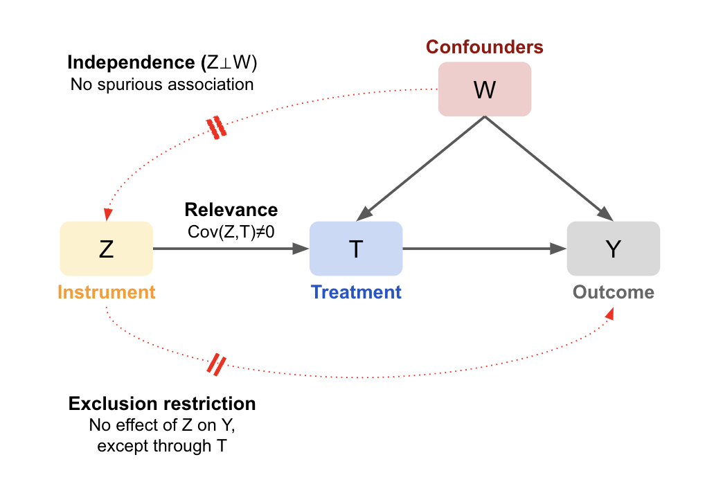
Key assumptions:
- Relevance: The instrument Z has a non-zero causal effect on the treatment T (Z->T), meaning \(Cov(Z,T) \neq 0\). Intuitively, Z needs to move T enough for us to see the change in Y. This assumption is testable.
- Exclusion Restriction: Z affects Y only through T, meaning there’s no direct or indirect effect of Z on Y, so we can assume any change in Y is due to T. This is not testable, so it must be justified theoretically.
- Independence (exchangeability) (also called Ignorability / Instrument Exogeneity): The instrument is as good as randomly assigned with respect to Y, meaning there’s no open backdoor paths that could cause a spurious correlation. Given there are unmeasured confounders, this is not testable with data, so it also must be justified theoretically.
- Monotonicity: The effect of T on Y must be homogenous (only in one direction) and linear (in the case of a binary treatment this is guaranteed) to interpret it as a Local Average Treatment Effect (LATE). Meaning the estimates are specific to those who were shifted by the instrument (from Y=0 to Y=1, known as compliers). The never-takers and always-takers are unchanged (\(T_\text{i0}=T_\text{i1}\)), so IV says nothing about the effect for them. Though uncommon, we assume there are no defiers (those who do the opposite).
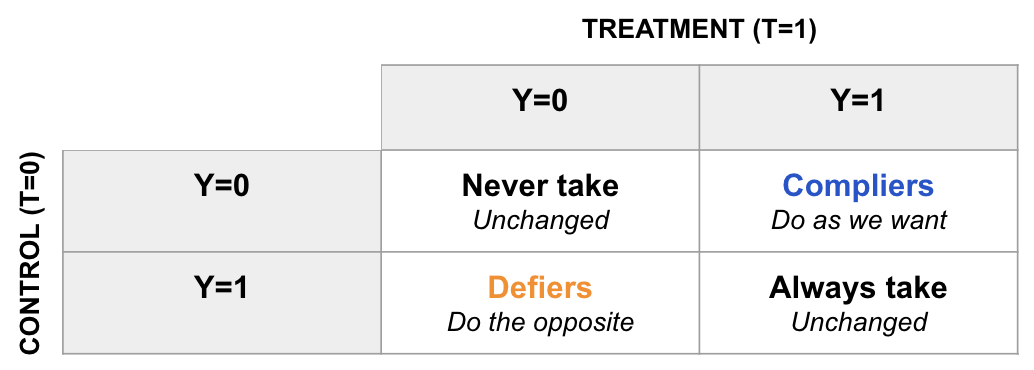
Monotonicity is considered optional because it’s not essential for the identification of the causal effect; rather, it affects the interpretation of the estimate. If monotonicity holds, you get a clean interpretation of the treatment effect as the LATE for the compliers. If the compliers are not special in any way, the results should generalise well to the whole population, but it’s not gauranteed like in a randomised experiment. If monotonicity doesn’t hold, the IV estimate becomes more complex, representing a weighted average of treatment effects (WATE) across different groups (rather than a uniform effect), making it harder to interpret and generalise.
How it works
As described above, the association of the instrument Z with the outcome Y will be a linear multiple of the association of the instrument Z with the treatment T:
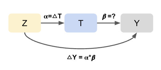
- First stage effect (α): Regress T on Z to estimate how much the instrument shifts the treatment (the part of T explained by Z). This gives the first-stage coefficient α, where a 1-unit increase in Z causes an α-unit change in T.
- Reduced-form effect (\(\Delta Y = α*β\)): Regress Y on Z to estimate the total effect of the instrument on the outcome. Since Z moves T by α, and T causes a change in Y by β, the overall change in Y due to Z is α⋅β. This is called the reduced form because it skips over the treatment step.
- Solving for β: Re-arranging the above formula gives us the effect of T on Y (β): \(\beta = \frac{\Delta Y}{\alpha} = \frac{\text{Reduced form}}{\text{First stage}}\).
Since IV estimates rely on marginal differences (i.e. changes in T and Y), we can (and should) use linear regression even if the outcome is binary or categorical. The goal is not to perfectly model Y, but to isolate variation in T that is exogenous (i.e. uncorrelated with confounders), using Z. Importantly, linear regression in the first stage (T ~ Z) ensures that we isolate the part of T that is orthogonal to unobserved confounders (the error).
Wald Estimator
For a single binary instrument and binary treatment, the Wald estimator directly applies the logic above:
\[\hat{\beta}_{\text{IV}} = \frac{E[Y \mid Z = 1] - E[Y \mid Z = 0]}{E[T \mid Z = 1] - E[T \mid Z = 0]} = \frac{\alpha \cdot \beta}{\alpha} = \frac{\text{Reduced form}}{\text{First stage}}\]If the instrument perfectly predicts treatment (i.e. 100% compliance), the denominator is 1, and the estimator reduces to the difference in outcomes (like a standard randomized controlled trial). However, if the instrument is weak (i.e. α is close to 0), the denominator becomes small, leading to unstable and biased estimates.
Two-stage least squares (2SLS)
In practice, 2SLS is the standard method for IV estimation (e.g. IV2SLS in Python’s linearmodels):
- First stage (\(\hat{T}\)): Same as before, regress T on Z. However, now we take the predicted treatment values as the output (\(\hat{T}\));
- Second stage (\(\beta\)): Regress Y on \(\hat{T}\) to isolate the component of T that is attributable to Z (i.e. removing variation), removing variation due to confounders.
In the simple case of one instrument and no covariates, 2SLS produces the same result as the Wald estimator. But unlike Wald, 2SLS extends to: multiple instruments; continuous treatments and instruments; the inclusion of control variables (added to both stages); and valid standard errors (accounts for the fact \(\hat{T}\) is an estimate and not an observed value).
Example
Let’s solidify this logic with a simplified example. Suppose we want to estimate the effect of ad exposure (T) on purchases (Y). A temporary bug (Z) in the ad system randomly caused some users to be 30 percentage points less likely to see ads (first stage effect: α=0.3). Those affected by the bug (Z=1) had a 1 percentage point lower conversion rate during the session (reduced form effect: α⋅β=0.01). This tells us that a 30 percentage point decrease in ad exposure leads to a 1 percentage point decrease in purchases. Using the Wald estimator to scale up, the effect of 100% of users not seeing ads is estimated as \(\frac{0.01}{0.3}=0.03\), meaning removing all ads would cause a ~3 percentage point drop in conversion.
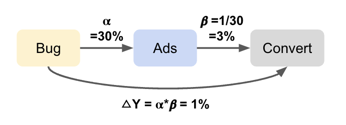
This is an overly simplified example: we assume all IV assumptions hold. In reality, we’d need to test exchangeability (e.g., did the bug disproportionately affect certain segments or device types? Are the periods comparable and generalizable? Could users have noticed the change and reacted differently?). If there are measurable confounders of Z and Y, we can add these as covariates in 2SLS (e.g. device type).
Selecting an instrument
Finding a valid instrument is challenging in practice. In industry, common sources of instruments include bugs, experiments (especially unrelated A/B tests that nudge compliance with treatment), feature rollouts, and external shocks such as policy changes or outages (i.e. natural experiments). While these are commonly available, recall they need to have a strong enough effect on the treatment to be viable (i.e. the first stage estimate must be significant). It’s also possible to use user, device, or product traits as instruments (e.g. OS type, app version), but these are often directly or indirectly correlated with outcomes of interest (e.g. conversion rates), violating the exclusion restriction.
Some examples of instruments for inspiration:
-
In this study a policy reform that raised the minimum school-leaving age was used as an instrument to estimate the effect of education on wages. Direct comparisons of students by years of schooling would be confounded by factors like ability. But assuming cohorts before and after the reform are comparable, and wages weren’t otherwise affected by the policy, the change in average earnings reflects the causal effect of an additional year of education.
-
At Uber (hypothetically) a bug was used as an instrument to study the effect of delivery delays on customer engagement. Comparing delayed vs. non-delayed orders is biased by factors like order volume. But if the bug randomly introduced delays and had no direct effect on engagement, it isolates the causal effect of delay.
-
Roblox used an old A/B test as an instrument to measure the effect of Avatar Shop engagement on community engagement. The test, originally designed to evaluate a recommendation feature, strongly influenced shop engagement but had no other impact on the platform—satisfying both relevance and exclusion.
-
At Booking.com, Account Managers (AMs) attempt to reactivate property partners who have left the platform. To measure the effect of these reactivation calls, a randomized encouragement design is used: some partners are randomly assigned to be contacted (instrument), but AMs retain discretion over whether to actually make the call (treatment). This setup introduces noncompliance, which prevents the use of traditional A/B testing to identify the causal effect of the call. Instead, the company applies the Instrumental Variable approach to estimate bounds on the Average Treatment Effect (ATE), relying on the random assignment as a valid instrument. This method accounts for the reality that AMs do not always follow assignments, while still enabling Booking.com to draw meaningful, data-driven conclusions about the value of outreach efforts.
-
Another common example is using an experiment as an instrument to correct for non-compliance. Suppose the treatment is a pop-up banner designed to encourage conversion, but on some devices it doesn’t appear due to ad blockers. This creates non-compliance: some users assigned to treatment don’t actually receive it. The estimated treatment effect (intent-to-treat effect) will be attenuated (biased towards 0), since it includes users who didn’t receive the treatment. By using treatment assignment as the instrument and actual treatment received as the treatment variable, we can recover the local average treatment effect (LATE) for compliers: those whose treatment status was influenced by assignment (e.g. users without ad blockers). This addresses the potential confounding of treatment received (e.g. if tech-savvy or higher-income users are more likely to block ads). If non-compliance is actually random, LATE should generalize to the full population, and we recover the average treatment effect (ATE). A variation of this example is when you over-expose an experiment, and want to measure the effect only on a subset of the population.
Multiple instruments
A core limitation of IV analysis is that it estimates the causal effect for the compliers (LATE), i.e. individuals whose treatment status is influenced by the instrument Z. Since different instruments influence different subsets of the population, LATEs can vary across studies or contexts. This raises an important question: how representative is a given LATE of the true Average Treatment Effect (ATE) for the broader population? One strategy to address this is to use multiple, independent instruments. Each instrument identifies a LATE for its own set of compliers. By collecting these localized causal effects, we can explore how treatment effects vary across subgroups, and, under certain conditions, approximate the ATE by combining them.
Two main approaches: Joint model (multiple instruments together): Include all instruments simultaneously in the model. This produces a weighted average of the LATEs, where weights reflect each instrument’s first-stage strength (i.e. how strongly it shifts the treatment). All instruments must be valid (satisfying relevance and exclusion). For example, Angrist & Krueger (1991) combined quarter of birth (affects students on the margin of school-entry age) and compulsory schooling laws (affects those who would have dropped out without the law) to instrument for education, leveraging variation in both school entry and legal leaving age.
- Separate models (one per instrument): Estimate separate IV models using one instrument at a time. This allows more flexibility in reporting heterogeneity in treatment effects across subpopulations. You can then combine the estimates using weighted averages. Weights might reflect sample size, inverse variance (as in meta-analysis), or instrument strength (e.g. Cov(T,Z)). For example, you might use several independent past experiments as instruments.
However, averaging multiple LATEs doesn’t guarantee you recover the ATE. As an analogy: each LATE is like a torch illuminating one part of a room. To reconstruct the full picture (the ATE), you either need to shine lights in the right places or understand the room’s layout. You can only recover the ATE if one of the following is true:
- Treatment effects are homogeneous: If the treatment has the same effect for everyone, then the LATE equals the ATE, no matter who the compliers are; or
- Compliers are representative of the full population: If the compliers have the same distribution of treatment effects as the overall population, then even if effects vary, the average effect for compliers still matches the ATE; or
- You can model heterogeneity explicitly: If you can model how treatment effects vary across individuals, and know who the compliers are for each instrument, you can “piece together” the ATE using the appropriate weights or adjustments (e.g. using covariates, interaction terms, hierarchical models, or meta-regression).
In practice, compliers often differ systematically. They may be more persuadable, more marginal, or behave differently in ways that affect treatment response. Understanding and adjusting for these differences is essential when trying to generalize from LATEs to broader conclusions.
Adding Covariates
Additional covariates are often necessary to satisfy identifiability assumptions when using observational instruments (e.g. adding confounders of the instrument Z and the outcome Y to both stages in 2SLS). However, this does not estimate the Local Average Treatment Effect (LATE) conditional on those covariates. Instead, the result is a weighted average of conditional LATEs, where the weights are determined by how the instrument varies across covariate strata and how those strata relate to the outcome. If treatment effects are heterogeneous across strata, or if defiers are present, these weights can become non-intuitive. They may be negative, exceed one, or fail to reflect subgroup sizes or first-stage strength. As a result, even with a valid instrument, the IV estimate \(\beta\) can be distorted and difficult to interpret as the effect for any specific population subgroup.
To address this, Słoczynski (2024) proposes two remedies:
- Use multiple instruments and test for consistency across estimands using overidentification tests (for example, Hansen’s J test). If the instruments are valid and identify the same causal effect, the estimates should agree.
-
Reordered IV: Remove the influence of covariates by residualizing each variable with respect to X, then perform IV on the residualized variables:
\(\tilde{T} = T - \mathbb{E}[T \mid X]\) \(\tilde{Z} = Z - \mathbb{E}[Z \mid X]\) \(\tilde{Y} = Y - \mathbb{E}[Y \mid X]\)
Then estimate:
\(\tilde{T} = \alpha \tilde{Z} + \varepsilon_T\) \(\tilde{Y} = \gamma \tilde{Z} + \varepsilon_Y\) \(\beta = \frac{\gamma}{\alpha} = \frac{\text{Cov}(\tilde{Y}, \tilde{Z})}{\text{Cov}(\tilde{T}, \tilde{Z})}\)
This approach ensures the final estimate reflects a cleaner average of the conditional LATEs, one where the weights depend only on the distribution of the covariates, not their relationship to the instrument or outcome.
Bias
Even with a valid instrument, a weak correlation between Z and T leads to noisy and potentially biased IV estimates. When the instrument is weak, the first-stage regression poorly predicts the treatment (\(\hat{T}\)). Although the noise is symmetric, the estimated first-stage coefficient can be close to zero or even change sign. Since the IV estimator can be expressed as \(\hat{\beta} = \frac{Cov(Z,Y)}{Cov(Z,T)}\), dividing by a small or near-zero denominator causes the estimate to “blow up,” producing a few extremely large positive outliers. Sensitivity tests are therefore important, because even small violations of the assumptions can result in a large bias. Importantly, the direction of the bias in IV estimates typically matches that of OLS. For example, if confounders are positively related to the treatment but negatively related to the outcome, both OLS and IV estimates will underestimate the true effect (negative bias).
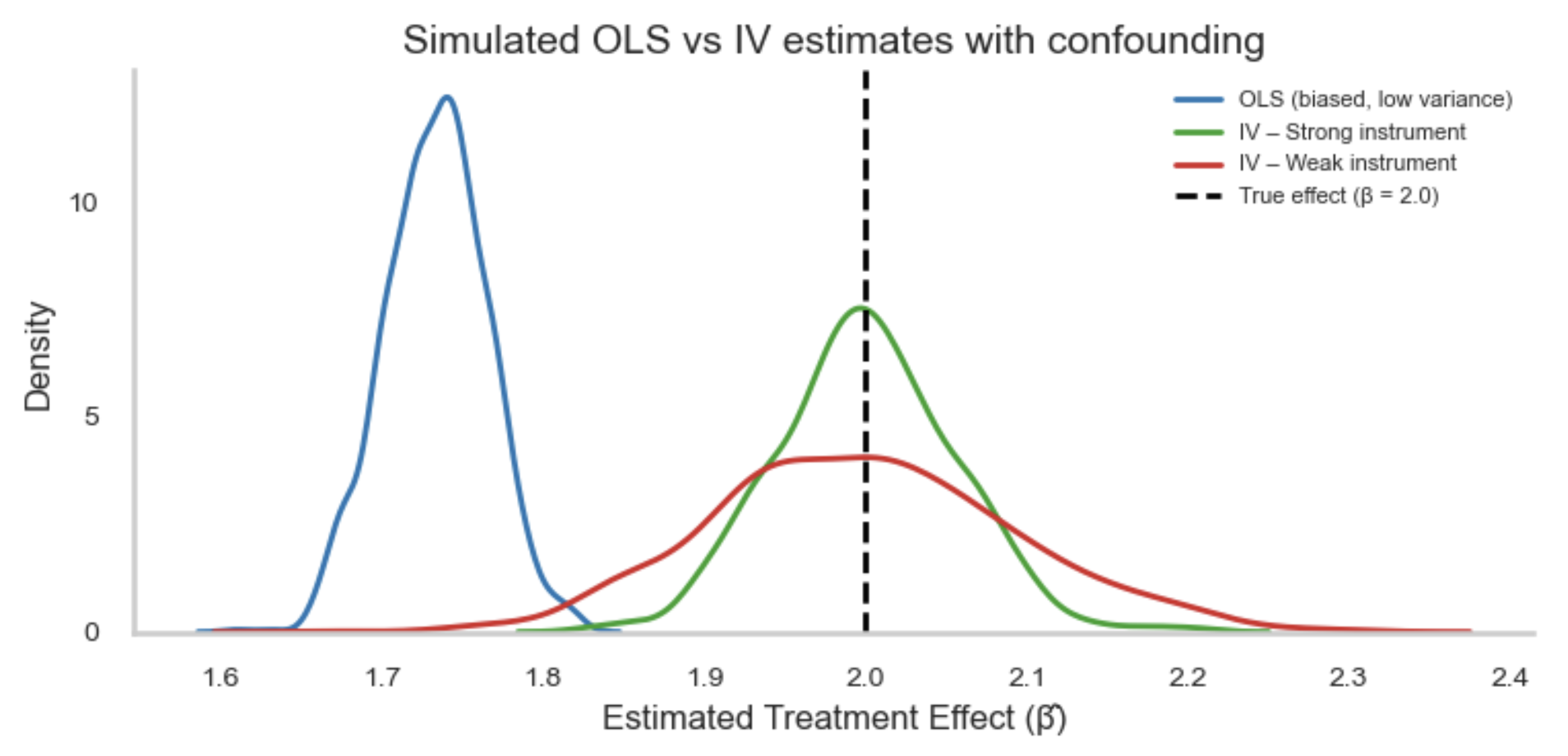
However, IV is consistent, meaning it will approach the population value as the sample increases. Whereas, under confounding, the OLS estimate remains biased:
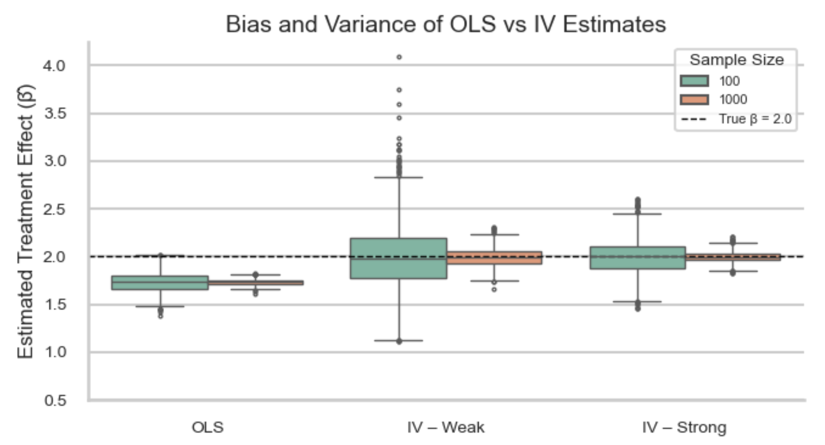
Deep IV
Deep IV is a method that extends instrumental variable (IV) analysis to handle nonlinear relationships and heterogeneous treatment effects using deep learning. It addresses the limitations of traditional IV approaches like Two-Stage Least Squares (2SLS), which assume linearity and constant treatment effects. Instead of fitting simple linear models, Deep IV uses neural networks to flexibly model the treatment and outcome processes in two stages:
-
Stage 1: Model treatment assignment given the instrument A neural network learns a conditional distribution of the treatment given the instrument and covariates, capturing how the instrument influences treatment across different subgroups in the data:
\[p(T \mid Z, X)\] -
Stage 2: Model the outcome Another neural network learns the causal relationship between the treatment, covariates, and outcome:
\[h(T, X)\]Instead of using observed treatment values directly, the model integrates over the predicted treatment distribution from Stage 1 to minimize a counterfactual loss to ennsure it captures exogenous variation in treatment due to the instrument, not variation that might be confounded:
\[\mathbb{E}_{T \sim p(T \mid Z, X)} \left[ L(h(T, X), Y) \right]\]
It can be especially useful in settings with high-dimensional data, such as personalized recommendations, pricing strategies, or policy evaluation. However, it still relies on the standard IV assumptions (exclusion restriction and instrument relevance), requires careful tuning, and can be computationally expensive.
Causal strength
The ideal setting for IV is more restrictive than other methods. However, when a strong instrument is available, IV can be a powerful tool. It enables estimation of causal effects even when unmeasured confounding is present, and can also handle issues like simultaneity bias (feedback loop) and measurement error in the treatment (if uncorrelated with the instrument). However, IV relies on a distinct set of assumptions that are largely theoretical and often untestable, so the credibility of any causal claims hinges on their plausibility in the specific context.
- Exchangeability (independence and exclusion restriction): Instead of assuming that the treatment T is independent of the potential outcomes Y (which fails in the presence of unmeasured confounders), IV analysis assumes that the instrument Z affects the outcome Y only through its effect on T. That is, Z must be conditionally independent of Y given T (i.e., no direct or confounding paths from Z to Y). This is known as the exclusion restriction and is not testable with data.
- Positivity (overlap): The instrument Z must exhibit sufficient variation across the population (i.e. we observe both values of Z) and must have a strong enough effect on the treatment T. This ensures that changes in Z induce observable changes in T, which in turn generate variation in Y. Weak instruments violate this and lead to imprecise or biased estimates.
- Consistency: IV assumes well-defined and stable treatments and instruments, and that each unit’s outcome reflects the treatment they actually received. Violations can arise if the instrument operates inconsistently, affects the outcome through unintended channels, or interferes across units.
These assumptions mean IV is best for cases where there’s a lot of unmeasured confounding, a binary and time fixed treatment, and a strong instrument. Further, the effect should be homogenous, or you are truly interested in the effect in the compliers, and monotonicity holds.
Difference in differences
Difference-in-Differences (DiD) is another quasi-experiment technique used to estimate causal effects when we observe outcomes before and after a treatment for both a treated and control group. It is especially useful for macro-level interventions such as policy evaluations (e.g. assessing the effect of a new law on unemployment) or marketing campaigns that lack granular tracking (e.g. TV ads or billboards). It would be a mistake to simply compare outcomes before and after the intervention in the treated group alone, as this ignores other time-varying factors unrelated to treatment that may have affected the outcome (e.g. seasonality, any underlying trend). The control group serves as a counterfactual, showing what would have happened to the treated group had the intervention not occurred. However, we also can’t just compare the treated and control group at the post treatment time period either as there can be pre-existing differences. To get around this, we look at the difference between the pre-post difference of each group (cancelling out any pre-existing difference between the groups by comparing groups, and cancelling out any time invariant confounders by comparing time periods). The key assumption is that, in the absence of treatment, both groups would have followed parallel trends. If that’s true, then any divergence in outcome trends after treatment can be attributed to the treatment effect.
Suppose we have two time periods: pre-treatment (t=0) and post-treatment (t=1); and, two groups: treated (D=1) and control (D=0). Using potential outcomes notation, we can write these as \(Y_D(t)\) (e.g. \(Y_1(0) \mid D=1\) is the potential outcome under treatment before treatment is implemented, averaged among those who were actually treated).
Using this notation, the DiD estimator (ATT) is:
\[\hat{ATT} = \left( \mathbb{E}[Y_1(1) \mid D=1] - \mathbb{E}[Y_0(1) \mid D=0] \right) - \left( \mathbb{E}[Y_1(0) \mid D=1] - \mathbb{E}[Y_0(0) \mid D=0] \right)\]Where:
- \(\mathbb{E}[Y_1(1) \mid D=1]\) is observed and estimated by \(\overline{Y}_{\text{treated, post}}\)
- \(\mathbb{E}[Y_0(1) \mid D=0]\) is the unobserved treated counterfactual, estimated by \(\overline{Y}_{\text{control, post}}\)
- \(\mathbb{E}[Y_1(0) \mid D=1]\) is the unobserved control counterfactual, estimated by \(\overline{Y}_{\text{treated, pre}}\)
- \(\mathbb{E}[Y_0(0) \mid D=0]\) is observed and estimated by \(\overline{Y}_{\text{control, pre}}\)
Re-arranging the formula to group the treated and control terms, we switch to the observed outcomes to get the Difference-in-Differences (DiD) formula:
\[\widehat{\text{DiD}} = \big(\overline{Y}_{\text{treated, post}} - \overline{Y}_{\text{treated, pre}}\big) - \big(\overline{Y}_{\text{control, post}} - \overline{Y}_{\text{control, pre}}\big)\]To estimate what would have happened to the treated group if they hadn’t been treated (the counterfactual), we’re taking the pre-treatment average for the treated group, and adding the change observed in the control group (since they weren’t treated):
\[\mathbb{E}[Y_0(1) \mid D = 1] = \overline{Y}_{\text{treated, pre}} + \left( \overline{Y}_{\text{control, post}} - \overline{Y}_{\text{control, pre}} \right)\]Regression
While you only need the group averages for the DiD formula above, converting it to a regression allows us to easily compute the standard error and confidence intervals. For this we need granular data (i.e. one row for each unit i and time period t). Using \(\text{Post}_t\) to indicate the time period (1 if after treatment, 0 if before), and \(\text{Treated}_i\) to indicate treatment (1 if unit i is in the treated group, 0 otherwise), we get:
\[Y_{it} = \alpha + \beta \cdot \text{Post}_t + \gamma \cdot \text{Treated}_i + \delta \cdot (\text{Treated}_i \times \text{Post}_t) + \varepsilon_{it}\]Where:
- \(Y_{it}\): Outcome for unit i at time t
- \(\alpha\): Intercept (the average outcome for the control group in the pre-treatment period, i.e. when both Post = 0 and Treated = 0).
- \(\beta\): The average change in outcome for the control group from pre-treatment to post-treatment (i.e. Post=1, Treated=0). This captures time trends common to both groups (e.g. seasonality, inflation).
- \(\gamma\): The difference in outcomes between the treated and control groups pre-treatment (i.e. Post=0, Treated=1). This reflects any time-invariant baseline differences between the two groups.
- \(\delta\): The interaction term only equals 1 for the treated group after treatment (i.e. Post=1, Treated=1). Therefore, it estimates how much more (or less) the treated group changed from before to after treatment, relative to the control group (i.e. any extra change in the treated group after controlling for the general time trends and baseline differences). This is the DiD estimator, the average treatment effect on the treated (ATT).
- \(\varepsilon_{it}\): Error term (unobserved factors)
Coming back to the DiD formula, we’re estimating the four group means from the model:
| Group | Post_t | Treated_i | Interaction | Expected Y |
|---|---|---|---|---|
| Control, Pre | 0 | 0 | 0 | $\alpha$ |
| Control, Post | 1 | 0 | 0 | $\alpha + \beta$ |
| Treated, Pre | 0 | 1 | 0 | $\alpha + \gamma$ |
| Treated, Post | 1 | 1 | 1 | $\alpha + \beta + \gamma + \delta$ |
Then we can do the same subtractions as before to get the DiD estimator:
\[\widehat{\text{DiD}} = \big(\overline{Y}_{\text{treated, post}} - \overline{Y}_{\text{treated, pre}}\big) - \big(\overline{Y}_{\text{control, post}} - \overline{Y}_{\text{control, pre}}\big)\]To visualise what we’re doing, let’s create the counterfactual line by adding \(\gamma\) (i.e. the difference between treated and control at the pre-treatment time point) to the control line. This assumes the growth in the control is the same as the treated would have been had they not received treatment. The gap between the counterfactual and the observed value for the treated at the post-treatment time point is our DiD estimate \(\delta\) (ATT).
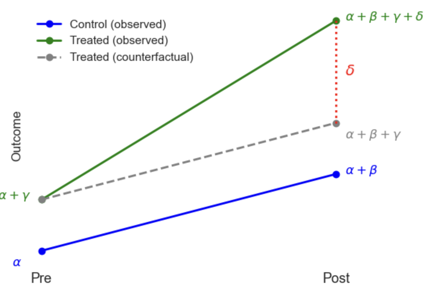
To show how this is differencing out unobserved confounders that are constant over time, suppose the true data-generating process is:
\[Y_{it} = \alpha_i + \gamma_t + \delta D_{it} + \varepsilon_{it}\]Where:
- \(\alpha_i\) captures all unit-specific effects (e.g. innate characteristics, geography, etc.)
- \(\gamma_t\) captures time effects common to all units (e.g. inflation, a new law, seasonality)
- \(D_{it}\) is the treatment indicator (1 if unit \(i\) is treated at time \(t\))
- \(\delta\) is the treatment effect of interest
- \(\varepsilon_{it}\) is an idiosyncratic error (noise or residual variation that is specific to an individual unit and time, but not systematically related to treatment or time)
By looking at differences over time within units, DiD cancels out \(\alpha_i\) (the time-invariant characteristics), because they don’t change between periods. Then, by comparing across groups, it cancels out \(\gamma_t\) (the common time based effects), as long as both groups are equally affected. This leaves just the treatment effect (\(\delta\)) and noise (\(\varepsilon\)). However, given we assume parallel trends in the absence of treatment, it does not remove bias from time-varying confounders that affect the groups differently (e.g. one group improves faster over time regardless of treatment).
Example
Suppose a new education policy (e.g. a new curriculum) is implemented only in one school zone, beginning in year t=1. You want to evaluate the impact of this policy on student test scores. Students are observed over time in both the treated and control zones.
\[Y_{it} = \alpha_i + \gamma_t + \delta D_{it} + \varepsilon_{it}\]- \(Y_{it}\) = Test score for student \(i\) at time \(t\)
- \(D_{it}\) = 1 if student \(i\) is in the treated zone after the policy is implemented (i.e., post-treatment), 0 otherwise
- \(\alpha_i\): Captures student- or school-specific fixed effects (do not change over time), such as:
- School zone characteristics (e.g., average income, teacher quality)
- Baseline differences in student ability or parental education
- Geographic or demographic differences
- \(\gamma_t\): Captures year-specific shocks common to all zones, such as:
- Changes to the national curriculum or test format
- Macroeconomic conditions
- COVID-19 disruptions or weather-related school closures in year \(t\)
- \(\delta D_{it}\): The causal effect of the education policy, i.e., the average treatment effect on the treated (ATT) — this tells us how test scores changed due to the policy in the treated zone, above and beyond what would have happened without the policy.
- \(\varepsilon_{it}\): The idiosyncratic error term, capturing random or unobserved student-specific shocks that vary over time:
- The student had a bad day or was sick during the test
- A fire drill interrupted the exam
- Random variation in scoring or guessing
Extensions
Covariates: You can add observed covariates to the DiD model to improve precision or adjust for time-varying confounding (any residual imbalance in characteristics that change over time and differ across groups). This doesn’t change the identifying assumptions but helps reduce residual variance (narrower confidence intervals). Below, \(\mathbf{X}_{it}\) is the vector of covariates and \(\mathbf{\beta_3}\) are the corresponding coefficients:
\[Y_{it} = \beta_0 + \beta_1 \text{Post}_t + \beta_2 \text{Treated}_i + \delta \big(\text{Treated}_i \times \text{Post}_t\big) + \mathbf{\beta_3} \mathbf{X}_{it} + \epsilon_{it}\]Multiple time periods: The classic DiD setup compares two time points: pre-treatment and post-treatment. But DiD is easily generalized to panel data with multiple time periods. This lets you see how the treatment effect evolves over time — before and after treatment. Instead of one single \(\delta\), you have a vector of treatment effects \(\delta_\tau\) indexed by time since treatment:
\[Y_{it} = \alpha_i + \gamma_t + \sum_{\tau \geq 0} \delta_\tau \cdot 1(t = \tau) \cdot D_i + \boldsymbol{\beta} \mathbf{X}_{it} + \epsilon_{it}\]- \(\alpha_i\) and \(\gamma_t\) are still your fixed effects for units and time.
- \(D_i\) is a simple indicator that unit \(i\) ever receives the treatment (e.g., treated school districts).
- \(1(t = \tau)\) is an indicator variable that equals 1 if the current time period \(t\) is exactly \(\tau\) periods after the treatment started.
- The product \(1(t = \tau) \cdot D_i\) is thus 1 only for treated units at exactly \(\tau\) periods after treatment.
- \(\delta_\tau\) is the treatment effect specific to the \(\tau\)-th post-treatment period.
Say you have data for 3 years after treatment starts (\(\tau\) =0,1,2):
- \(\delta_0\) measures the immediate impact of treatment in the first period.
- \(\delta_1\) measures the effect in the second period after treatment.
- \(\delta_2\) measures the effect in the third period after treatment.
By estimating separate \(\delta_\tau\) for each year, you can see whether the trend. For example it may: peak immediately and decline; build up gradually; remain stable; or behave in some other pattern. This richer model is often called an event study or dynamic DiD because it studies the evolution of treatment effects over time.
Assumptions:
Parallel Trends:
The key identifying assumption of Difference-in-Differences (DiD) is that, in the absence of treatment, the average outcome for the treated group and the control group would have followed the same trend over time. Formally, if we let \(Y_{it}(0)\) be the potential outcome without treatment for unit \(i\) at time \(t\), then:
In other words, we assume we can use the control as the counterfactual, so any differences in outcomes between treated and control groups before the treatment persist but do not change over time. If this assumption fails (e.g. treated group is on a systematically different trajectory), the DiD estimate will be biased. In industry this is often an issue because the choice of who to treat is targeted (e.g. testing a new feature in a lower performing market to try improve it). In practice, we might find a control by plotting pre-treatment trends in the outcome for each potential control vs the target group. If they appear parallel before treatment, the assumption is more credible:
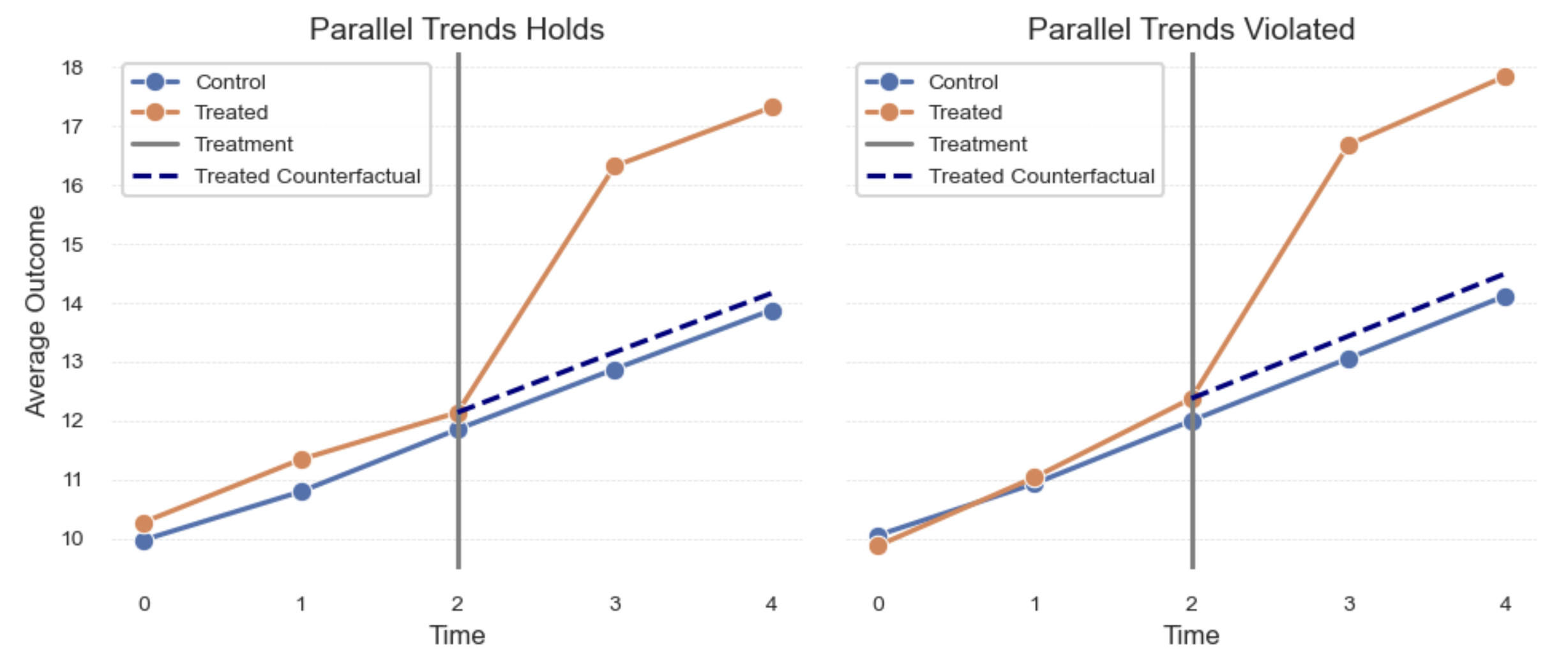
In addition to eyeballing it, we can fit a regression on the pre-treatment time period, using interaction terms (Treated x Time) to assess whether there is a pre-treatment difference in the slopes. Starting with a simple case of two time periods pre-treatment:
\[Y_{it} = \beta_0 + \beta_1 \, \text{Treated}_i + \beta_2 \, \text{Time}_t + \beta_3 \, (\text{Treated}_i \times \text{Time}_t) + \varepsilon_{it}\]| Term | Value | Coefficient | Meaning |
|---|---|---|---|
| $\text{Treated}_i$ | 1 if unit $i$ is treated, 0 otherwise | $\beta_1$ | Measures the average difference in outcomes between treated and control groups at time = 0 (the baseline period). |
| $\text{Time}_t$ | 1 if time = 1 (later pre-period), 0 if time = 0 (baseline) | $\beta_2$ | Measures the average change in outcomes from time 0 to time 1 for the control group — that is, the baseline trend in the absence of treatment. |
| $\text{Treated}_i \times \text{Time}_t$ | 1 only if unit is treated and time = 1 | $\beta_3$ | Measures the difference in trends from time 0 to 1 between treated and control groups. Specifically, it compares the change for treated units to that for control units. A non-zero value means the groups had different trends before treatment — violating the parallel trends assumption. |
In this case, we could just use the t-test results for \(\beta_3\) to assess whether there is a significant difference. However, we can generalise this to multiple time periods and use an F-test to check if any of the interactions are significant:
\[Y_{it} = \beta_0 + \beta_1 \text{Treated}_i + \sum_{t=1}^T \beta_{2t} \, \text{Time}_t + \sum_{t=1}^T \beta_{3t} \, \big(\text{Treated}_i \times \text{Time}_t\big) + \varepsilon_{it}\]Where:
- \(\text{Treated}_i = 1\) if unit \(i\) is treated, 0 otherwise,
- \(\text{Time}_t\) are dummy variables for each time period \(t\), with the base period \(t = 0\) omitted,
- \(\text{Treated}_i \times \text{Time}_t\) are the interaction terms for treated units in time period \(t\),
- \(\beta_{3t}\) coefficients test whether the treated group’s trend differs from control’s in period \(t\) relative to the base period.
In Python, after identifying the names of the interactions, you can write the hypothesis (\(H_0: \beta_{31} = \beta_{32} = \cdots = \beta_{3T} = 0\)) as a string and pass it to f_test in statsmodels (to restrict the test to only the interactions). If it’s significant, this indicates a violation of the assumption. If there are many pre-treatment time periods, one option is to aggregate them, or pick certain lags (e.g. -1 month, -2 months). However, keep in mind this is only checking if they were parrallel pre-treatment and doesn’t rule out a difference in the post-treatment time period that is unrelated to treatment.
No Spillovers (Stable Unit Treatment Value Assumption - SUTVA):
The treatment assigned to one unit (e.g. one school zone) does not affect the outcomes of units in the control group. For example, if the new education policy in the treated zone indirectly improves resources or student outcomes in the control zone, this assumption is violated, potentially biasing estimates. This is harder to assess directly from the data, and relies instead on being familiar with the intervention and outcomes.
No Composition Change (No Differential Attrition or Migration):
The composition of the treated and control groups remains stable over time, and changes in group membership are not related to the treatment. For example, if after the policy starts, higher-performing students move into the treated zone (or control zone students move away), the comparison groups are no longer comparable, and the DiD estimator may be biased. If you have stable IDs over time, you can catch this by checking if any units are assigned to multiple treatments.
Causal strength
DiD is not suitable for all cases, but offers a simple way to control for unobserved, time-invariant confounders and common shocks when we have panel data (measurements over time), and the assumptions are plausible.
- Exchangeability (parallel trends): In DiD, instead of assuming that the treatment D is independent of the potential outcomes Y (which fails in the presence of unmeasured confounders), DiD assumes that, in the absence of treatment, the treated and control groups would have followed parallel trends (i.e. the growth in potential outcomes is independent of treatment assignment). This weaker assumption allows for unobserved confounding, as long as it is constant over time and affects both groups similarly (so it will get cancelled out).
- Positivity (overlap): Each group must have a positive probability of being observed both before and after the intervention. This means the groups must be present and measurable in all relevant time periods—otherwise we cannot estimate the group-specific trends needed for DiD.
- Consistency: The observed outcome for a unit under the treatment received and time period observed reflects the potential outcome for that treatment-time combination. Meaning: we are seeing the correct potential outcome (SUTVA); we are seeing it for a stable set of units (no composition change); and, we’re measuring it accurately, without bias introduced by how outcomes are recorded or constructed.
DiD is generally best for situations where:
- Treatment is assigned at a group level or policy is rolled out at a known time.
- There is reliable longitudinal data on treated and control groups.
- The parallel trends assumption is plausible or can be tested with pre-treatment data.
- Unobserved confounding is largely time-invariant.
Two-Way Fixed Effects (TWFE)
TWFE is essentially a regression implementation of DiD that generalizes to more than two time periods, staggered treatment timing (units get treated at different times), and continuous treatment variables. By adding the unit itself as a control to the model (i.e. a binary variable for each ID), we control for all of the things that are fixed for a unit even if we can’t measure them (e.g. over a short time period a person’s IQ is likely unchanged).
The TWFE model is typically written as:
\[Y_{it} = \alpha_i + \lambda_t + \tau D_{it} + \varepsilon_{it}\]Where:
- \(Y_{it}\): Outcome for unit \(i\) at time \(t\)
- \(\alpha_i\): Unit fixed effect, controls for time-invariant characteristics of each unit
- \(\lambda_t\): Time fixed effect, controls for shocks common to all units in period \(t\)
- \(D_{it}\): Treatment indicator, 1 if unit \(i\) is treated at time \(t\), 0 otherwise
- \(\tau\): The treatment effect (what we aim to estimate)
- \(\varepsilon_{it}\): Error term capturing unexplained variation
When estimating this model in a regression, you don’t estimate \(\alpha_i\) and \(\lambda_t\) directly. Instead, they are encoded as dummy variables, dropping one to avoid perfect multicollinearity:
- \(\alpha_i\): For N units, you include n-1 dummy variables (unit2, unit3, …, unitN). These dummies capture any unit-specific, time-invariant differences in outcome levels (e.g. permanent differences across individuals or regions).
- \(\lambda_t\): For T time periods, you include t-1 dummy variables (time2, time3, …, timeT). These capture any period-specific shocks or trends that affect all units equally (e.g. economic trends or policy changes affecting everyone).
The resulting regression looks something like this:
\[Y_{it} = \tau D_{it} + \sum_{i=2}^{N} \beta_i \cdot \text{unit}_i + \sum_{t=2}^{T} \gamma_t \cdot \text{time}_t + \varepsilon_{it}\]Demeaning (Within Transformation)
In practice, to avoid adding n-1 dummy variables which could be very large, we can use a method called “demeaning”. When you include dummy variables in a regression, you’re estimating and removing their average effect (or conditional average if there’s additional covariates). De-meaning does exactly the same thing, but more efficiently: it subtracts the averages directly, without estimating a coefficient for each dummy.
Step 1: Compute Averages
- Unit (i) averages:
- Time (t) averages:
- Overall averages:
Step 2: Two-Way Demeaning
Create demeaned variables by subtracting the averages, which removes both \(\alpha_i\) and \(\lambda_t\). Regressing on unit dummies controls for unit averages, so subtracting the unit means is a manual but more efficient way of removing the effect:
-
Demeaned outcome: \(\tilde{Y}_{it} = Y_{it} - \bar{Y}_i - \bar{Y}_t + \bar{Y}\)
-
Demeaned treatment: \(\tilde{D}_{it} = D_{it} - \bar{D}_i - \bar{D}_t + \bar{D}\)
Step 3: Regress the demeaned outcome on the demeaned treatment
The de-meaning process yields the same estimate as running a full regression with one-hot dummies for each unit and time period:
\[\tilde{Y}_{it} = \tau \tilde{D}_{it} + \tilde{\varepsilon}_{it}\]| Component | Explanation |
|---|---|
| \(\alpha_i\) | Removed via subtracting unit average |
| \(\lambda_t\) | Removed via subtracting time average |
| \(\tau\) | Estimated by regressing demeaned \(Y_{it}\) on \(D_{it}\) |
Assumptions
There are the functional form assumptions:
- Treatment Effect Heterogeneity: If the treatment effect varies across time or units, the TWFE estimate τ can be a weighted average of different effects, with some weights being negative. This can lead to misleading conclusions, as shown in recent research (e.g., Goodman-Bacon decomposition).
- Linearity in the covariates;
- Additive fixed effects.
But also the strict exogeneity assumptions:
- Parallel Trends: In the absence of treatment, treated and control units would have followed the same trend over time. TWFE enforces this assumption implicitly through fixed effects.
- No time-varying confounders: TWFE can’t handle variables that change over time and differ systematically between treated and control units — unless you explicitly model those.
- No anticipation
- Past treatment don’t affect current outcome (no carryover)
- Past outcome don’t affect current treatment (no feedback)
Bias
Recent econometrics research showed that staggered DiD with TWFE is biased when treatment effects are heterogeneous (post-2018, notably Goodman-Bacon, Sun & Abraham, Callaway & Sant’Anna). This is especially problematic when different groups adopt treatment at different times (e.g., state policies rolled out in different years), or when treatment effects grow or shrink over time. These patterns are common in real-world interventions, for example, an e-commerce site rolling out a feature by country, with the effect of the feature taking time to fully materialize.
The core problem is that some units act as controls for others after they’ve already been treated, causing TWFE to assign negative weights to certain comparisons. If the treatment effect increases over time, this tends to bias the overall estimate downward; if the effect decreases over time, it biases the estimate upward. As a result, the TWFE estimate isn’t just a weighted average of the group-specific effects, it’s a distorted mix of comparisons that can even have the wrong sign if treatment effects vary enough.
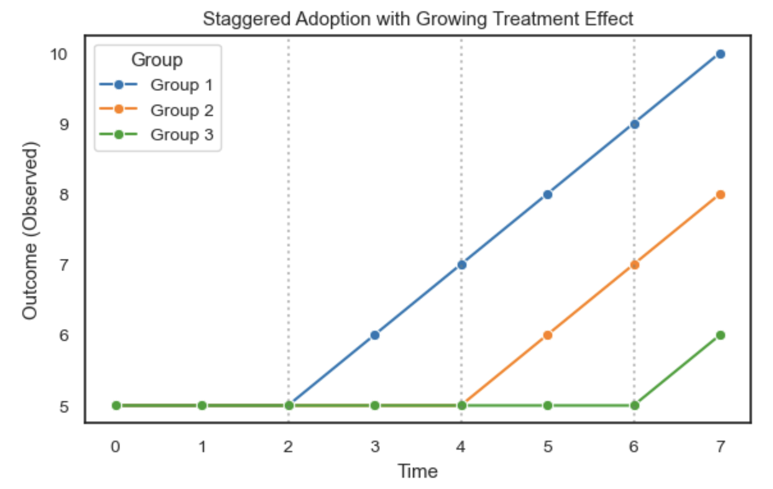
For staggered rollouts, researchers have increasingly moved toward more robust alternatives that explicitly model treatment effect heterogeneity, such as:
- Callaway & Sant’Anna (2021): Group-time average treatment effects.
- Sun & Abraham (2021): Interaction-weighted estimators correcting the TWFE bias.
- Gardner (2022) Did2s: A two-stage procedure that improves robustness in TWFE designs.
Using these approaches allows you to estimate group-specific treatment effects over time and avoid the misleading averages produced by naïve TWFE models in heterogeneous settings.
Causal strength
TWFE models extend DiD to more flexible settings with multiple time periods and variation in treatment timing. They offer a simple way to control for unobserved time-invariant confounders (via unit fixed effects) and time shocks common across units (via time fixed effects), using a linear regression framework.
- Exchangeability (parallel trends, conditional on fixed effects): Instead of assuming that treatment \(D\) is independent of potential outcomes \(Y\), TWFE relies on the assumption that, after removing unit and time fixed effects, treatment assignment is as good as random. In other words, in the absence of treatment, each unit’s outcome would have evolved similarly to others after accounting for fixed differences. This assumption allows for time-invariant unobserved confounding, as long as treatment timing is not systematically related to time-varying shocks.
- Positivity (overlap): There must be sufficient variation in treatment timing across units and time periods. That is, some units must be untreated while others are treated in each period (or across periods), so that treatment effects can be compared within the model. Without overlap, the model cannot identify treatment effects separately from unit or time effects.
- Consistency: The observed outcome \(Y_{it}\) equals the potential outcome \(Y_i(D_{it}, t)\). This requires:
- SUTVA (no interference between units, and a well-defined treatment),
- No composition change over time (units remain comparable),
- Reliable measurement of outcomes, with no differential measurement error by treatment or time.
TWFE is especially useful when:
- You have panel data with many time periods and staggered treatment adoption.
- You believe fixed differences between units and common time shocks are key confounders.
- Treatment varies within units over time (within-unit comparisons are possible).
- You want to estimate an average effect across units and time, accounting for these fixed effects.
Synthetic controls
Synthetic controls overcome the problem of finding a single good control for a DiD model. Instead of selecting one comparison unit, we take a weighted average of multiple control units to create a synthetic control that closely matches the treated unit’s trend during the pre-intervention period.
For example, imagine an e-commerce company runs a test for a new product in 1 of the 100 cities it operates in. Instead of choosing one comparison city, which may still not perfectly match the treated city, we construct a weighted combination of the remaining 99 cities to form a synthetic version. We then use this synthetic control as a proxy for what would have happened to the treated city post-intervention if it had not been treated.
Synthetic outcome formula
\[\hat{Y}^N_{1t} = \sum_{j=2}^{J+1} w_j Y_{jt}\]Where:
- \(\hat{Y}^N_{1t}\) is the synthetic (estimated) outcome for treated unit 1 at time \(t\)
- \(Y_{jt}\) is the outcome for control unit \(j\) at time \(t\)
- \(w_j\) is the weight assigned to control unit \(j\)
- \(\sum_{j=2}^{J+1} w_j = 1\) means the weights sum to 1 (convex combination)
- \(w_j \ge 0\) means the weights are non-negative
Finding the weights
The weights \(w_j\) are chosen to minimize the difference between the pre-treatment outcomes of the treated unit and its synthetic counterpart:
\[\min_{w} \sum_{t=1}^T \left( Y_{1t} - \sum_{j=2}^{J+1} w_j Y_{jt} \right)^2\]Where:
- \(Y_{1t}\) is the outcome for the treated unit at time \(t\) (pre-treatment)
- \(T\) is the number of pre-treatment periods
We can solve for these weights by running a regression where the units (for example, cities) are the features (columns) and the time periods are the observations (rows). However, this requires constrained least squares with:
- \[\sum_{j=2}^{J+1} w_j = 1\]
- \(w_j \ge 0\) for all \(j\)
These constraints ensure that the synthetic control stays within the range of observed data and avoids extrapolation.
Assessing significance: Placebo tests
Since we typically have few units (small sample size), standard errors from regression are unreliable. Instead, we use placebo tests:
- For each control unit, pretend it was treated, fit a synthetic control, and compute the resulting placebo effect.
- Compare the gap for the actual treated unit to the distribution of placebo gaps.
- The p-value is the proportion of placebo gaps that are larger than the estimated treatment effect.
This non-parametric test provides a practical way to assess whether the estimated treatment effect is meaningful or could plausibly have arisen by chance.
Bayesian structural time series
Another approach to estimating the effect of an intervention on time series data is Bayesian structural time series (BSTS), popularized by Google’s CausalImpact package.
Where synthetic controls build a weighted average of other units to form a comparison, BSTS builds a model-based forecast of what would have happened to the treated unit if the intervention had not occurred. It incorporates:
- Trends and seasonal patterns, capturing gradual movements or recurring cycles
- Covariates, control variables that help predict the outcome
- Uncertainty, using Bayesian inference to provide credible intervals for the estimated effects
The estimated effect of the intervention is calculated as the difference between the observed data and the predicted counterfactual in the post-treatment period.
Model structure
A typical BSTS model looks like this:
\[Y_t = \mu_t + \tau_t + \beta X_t + \epsilon_t\]Where:
- \(\mu_t\) is the local level, capturing gradual underlying trends
- \(\tau_t\) is the seasonal component, if applicable
- \(X_t\) represents observed covariates, such as control markets
- \(\beta\) are the coefficients for each covariate, estimated using spike-and-slab priors for automatic selection and regularization
- \(\epsilon_t\) is Gaussian random noise
The spike-and-slab priors are especially useful when there are many potential control variables. The spike controls whether a variable is likely to be included, while the slab shrinks included variables toward zero to guard against overfitting and multicollinearity.
How it works
- Fit the model on the pre-intervention period to learn patterns in the time series.
- Forecast the counterfactual to generate predictions for the post-intervention period, representing what would have happened without the intervention.
- Compare the observed data to the predicted counterfactual to estimate the causal impact.
- Quantify uncertainty using Bayesian credible intervals derived from the posterior distribution of the forecast.
Pre-selecting the control pool
While CausalImpact uses spike-and-slab priors to automatically select the most predictive control markets for the structural time series model, if you have many potential controls it can be useful to first reduce the pool to more viable candidates. Pre-selecting the control pool improves computational efficiency, reduces noise from unrelated markets, and can help avoid issues with multicollinearity between highly correlated controls.
One practical approach is to select control markets that have demonstrated similar trends to the treated market during the pre-intervention period. Similarity can be measured using methods like:
- Correlation or R-squared between time series
- Dynamic Time Warping (DTW), which allows for small temporal misalignments
- Distance metrics on smoothed or detrended series
The MarketMatching package, developed by Stitch Fix, provides a convenient implementation of this idea. It uses DTW to score similarity between time series and select a subset of controls with trends closest to the treated unit. These selected markets can then be used as covariates in the CausalImpact model.
After pre-selecting controls, it’s still important to validate the model by testing its performance on placebo interventions in the pre-treatment period. This helps ensure that the final model is well-calibrated and reduces the risk of detecting spurious effects.
Interpreting the results
By default, CausalImpact produces a three-panel plot:
- Observed versus predicted, showing the actual series against the counterfactual forecast
- Pointwise impact, the estimated effect at each time point
- Cumulative impact, the running total of the effect over time
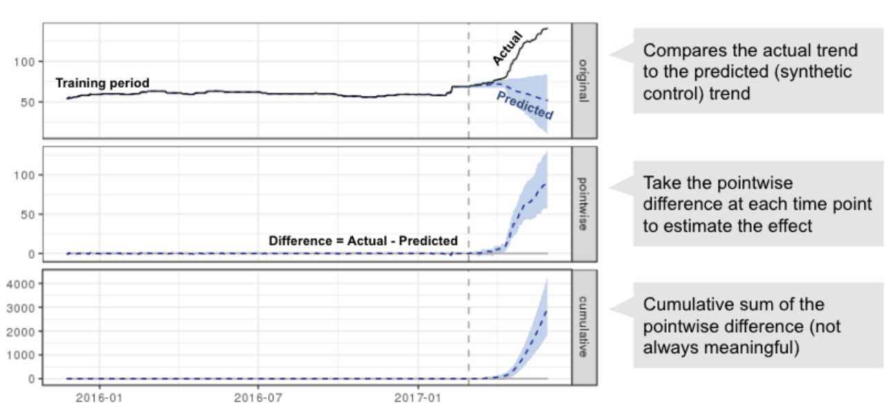
Cumulative impact is most meaningful when the outcome represents a flow, such as daily sales. For metrics defined at a point in time, like the number of customers, the pointwise impact is often more interpretable.
Benefits
- Models rich time series dynamics, including trends, seasonality, and covariates
- Provides uncertainty intervals for effect estimates
- Supports automatic variable selection when many potential controls are available
- Well-suited for cases with a single treated unit and a long pre-intervention time series
Limitations
- Relies on the pre-intervention model being well specified; at least 1.5 years of pre-period data is recommended for robustness, especially if cross-validation is used
- Structural breaks or confounding changes after the intervention can bias estimates. Limiting the post-treatment period, for example to one month, can reduce this risk
- Requires more modeling choices than simpler approaches like Difference-in-Differences or synthetic controls
- Frequentist inference is not directly available. Statistical significance is assessed using Bayesian posterior probabilities instead of p-values
Testing robustness
To assess robustness, placebo tests can be used:
- Simulate “fake” interventions during the pre-treatment period
- Fit the model and check how often it detects a significant effect when no intervention actually occurred
- Use this to estimate the model’s false positive rate and tune parameters like the number of control variables and prior assumptions
Choosing between DiD / synthetic control / BSTS
| Method | Best for | Key assumptions | Strengths | Limitations |
|---|---|---|---|---|
| Difference-in-Differences (DiD) | Many treated & control units with parallel trends | Parallel trends (or conditional on covariates) | Simple to implement, interpretable | Sensitive to trend differences, no flexible control selection |
| Synthetic Control | One treated unit, good set of comparison units | Treated can be approximated by weighted avg. of controls | Transparent, intuitive counterfactual | Requires good controls, limited flexibility in dynamics |
| Bayesian Structural Time Series (BSTS) | One treated unit, complex or noisy time series | Pre-period model well specified, stable covariate relationships | Rich time series dynamics, automatic control selection | More complex setup, relies on prior choices, sensitive to model misspecification |
Recommendation:
- Use DiD for larger panel data with multiple treated units.
- Use Synthetic Control when you have few treated units but good controls.
- Use BSTS (CausalImpact) when controls are noisy, or the treated series has trends and seasonality that need to be modeled explicitly.
Regression Discontinuity
Regression Discontinuity Design is a quasi-experimental method used for estimating causal effects when treatment is assigned based on a cutoff in a continuous variable (called the running variable or forcing variable). Given we’re looking at a limited time period, we assume that everything else affecting y changes smoothly at the the cutoff (continuity assumption), so any jump must be due to treatment. For example, if we decide anyone who scores above 80 on a test gets some reward, those who scored 80 are likely very similar to those who scored 81. Graphically, RDD looks like two regression lines, one on each side of the cutoff. The discontinuity (the jump) between those two lines at the cutoff is what we interpret as the causal effect of the treatment.
After centering the running variable, we can specify the Regression Discontinuity Design (RDD) model as:
\[Y_i = \alpha_0 + \alpha_1 \cdot \tilde{r}_i + \alpha_2 \cdot 1\{\tilde{r}_i > 0\} + \alpha_3 \cdot 1\{\tilde{r}_i > 0\} \cdot \tilde{r}_i + \varepsilon_i\]Where:
- \(Y_i\): Outcome for individual \(i\)
- \(\tilde{r}_i = r_i - c\): Running variable centered at the cutoff \(c\), so that \(\tilde{r}_i = 0\) at the cutoff. This has 2 advantages: the intercept \(\alpha_0\) directly represents the expected outcome at the cutoff for the untreated group; and, the treatment effect \(\alpha_2\) is then interpreted as the causal effect of crossing the threshold.
- \(1\{\tilde{r}_i > 0\}\): Dummy variable, 1 if individual \(i\) is above the cutoff (treated), 0 otherwise
- \(1\{\tilde{r}_i > 0\} \cdot \tilde{r}_i\): Interaction term for the running variable and the cutoff dummy (allowing the slope to differ on either side of the cut-off)
- \(\varepsilon_i\): Error term
| Coefficient | Measures | Interpretation |
|---|---|---|
| $\alpha_0$ | Baseline (untreated) | Expected outcome at cutoff (coming from below) |
| $\alpha_1$ | Pre-cutoff slope | Trend of outcome as $r_i \to c^-$ |
| $\alpha_2$ | Treatment effect at cutoff | Causal estimate: jump when we switch on the dummy (\(\lim_{r_i \to c^+} \mathbb{E}[y_i \mid r_i] - \lim_{r_i \to c^-} \mathbb{E}[y_i \mid r_i]\)) |
| $\alpha_3$ | Change in slope due to treatment | Difference in slopes (change when the cutoff dummy switches to 1) |
With our running variable (centered at 0), cutoff dummy, and their interaction, we’re able to fit the pre and post cutoff slopes:
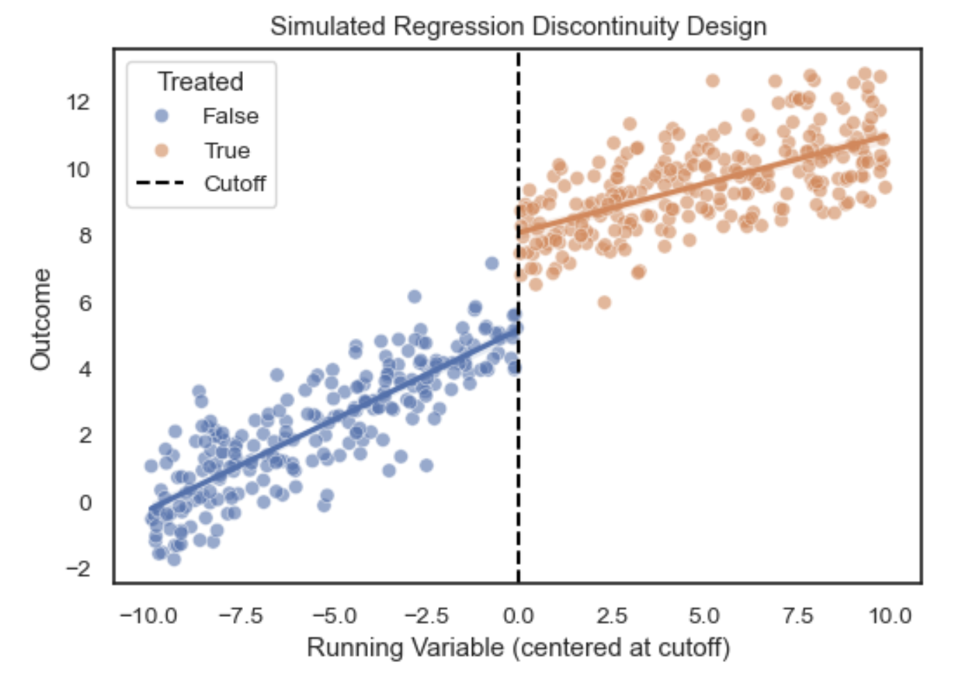
This can also be combined with earlier methods:
| RD Alone | RD + DiD (RDDiD) | RD + Matching/Covariates |
|---|---|---|
| Controls for confounding at the cutoff only. | Adds control for time trends in panel or repeated cross-section. | Improves covariate balance, reduces residual variance. |
| Local effect at the threshold. | Local difference in trends at the threshold. | Local effect, but more efficient. |
| You believe continuity in potential outcomes holds and no time trend confounding is likely. | There’s a policy or event at a specific time that might affect the groups even without treatment. | You see imbalance in covariates near the cutoff, especially with small samples. |
Diagnostics / improvements
Given we’re essentially fitting two regression slopes, it’s possible the model will focus too much on fitting all the points and not on the points at the cutoff (which is what our causal estimate measures). One solution to this is to give more weight to the points near the cutoff, emphasizing the part of the data most relevant for identifying the discontinuity. There are a few ways to do this:
- Kernel weighting: Use a kernel function (e.g., triangular, Epanechnikov) to assign higher weights to observations closer to the cutoff and lower weights to those further away. The triangular kernel is commonly used because it prioritizes points nearest the threshold.
- Bandwidth selection: The choice of bandwidth (how wide a window of data to use around the cutoff) is crucial. A smaller bandwidth reduces bias (focusing on near-cutoff observations) but increases variance (fewer data points). Larger bandwidths reduce variance but risk bias if the relationship between the running variable and the outcome is nonlinear. Data-driven methods (e.g., cross-validation, Imbens-Kalyanaraman) help select optimal bandwidths.
- Higher-order polynomials or local polynomial regression: Instead of simple linear models on either side of the cutoff, you can use quadratic or cubic terms, or fit local polynomial regressions, to better approximate the functional relationship within the chosen bandwidth. Care must be taken—overly flexible models can reintroduce bias by fitting noise.
- Covariate adjustment: While not required for identification, adding pre-treatment covariates can reduce residual variance and improve precision if these covariates are smoothly related to the running variable.
It’s good practice to try multiple bandwidths, kernels, and model specifications to check the sensitivity of your results.
McCrary Test
If units can precisely manipulate their position relative to the cutoff (e.g., by sorting or gaming eligibility), the assumption of continuity in potential outcomes may be violated, threatening identification. The McCrary test is a diagnostic for checking manipulation of the running variable around the cutoff. It tests whether there is a discontinuity in the density (distribution) of the running variable at the threshold by comparing densities just to the left and right of the cutoff. A significant jump suggests potential manipulation or sorting, while a smooth density supports the assumption that units cannot manipulate assignment precisely, strengthening the credibility of the RDD.
Causal strength
Under mild conditions (continuity of potential outcomes at cutoff), RD is as good as randomization near the threshold, making it very convincing when the assumptions hold. However, it only estimates the local average treatment effect (LATE) around the cutoff, not global effects (i.e. it doesn’t necessarily generalize to samples far from the cutoff).
- Exchangeability: Assumed to hold at the cutoff, because units just above and below the threshold are expected to be similar in both observed and unobserved characteristics. This hinges on the continuity of potential outcomes at the threshold.
- Positivity (overlap): Automatically satisfied near the cutoff, since we observe units on both sides of the threshold by design. However, treatment assignment is deterministic based on the running variable, meaning there’s local overlap, not global.
- Consistency: Requires that the treatment actually corresponds to the defined intervention at the threshold, and that there’s no interference between units (one unit’s treatment doesn’t affect another’s outcome).
Fuzzy RDD (non-compliance)
Standard (sharp) Regression Discontinuity Design (RDD) can be viewed as a special case of an Instrumental Variables (IV) design with perfect compliance at the cutoff. However, in many practical situations, treatment assignment is not perfectly determined by crossing the cutoff. Instead, the probability of receiving treatment increases discontinuously at the threshold, but some units above the cutoff might not receive treatment, and some below might receive it. This setting is known as fuzzy regression discontinuity design and can be estimated using an IV approach, where crossing the cutoff acts as an instrument for actual treatment receipt. The causal effect identified in fuzzy RDD is the local average treatment effect (LATE) for compliers, units whose treatment status is influenced by whether they cross the threshold.
- Let \(Z_i = \mathbf{1}(r_i \geq c)\) denote the instrument, indicating if the running variable \(r_i\) is above the cutoff \(c\).
- Let \(D_i\) be the actual treatment received by unit \(i\), which may not perfectly correspond to \(Z_i\) due to non-compliance or imperfect assignment.
- Let \(Y_i\) be the observed outcome for unit \(i\).
Because \(Z_i\) influences \(D_i\) only probabilistically, we use \(Z_i\) as an instrument for \(D_i\) to estimate the causal effect of treatment on the outcome:
First stage: Model the effect of the instrument on treatment assignment:
\[D_i = \pi_0 + \pi_1 Z_i + f(r_i) + \epsilon_i^D\]where \(f(r_i)\) flexibly models the relationship between the running variable and treatment (for example, separate slopes or polynomial terms on each side of the cutoff).
Second stage: Model the outcome as a function of predicted treatment:
\[Y_i = \beta_0 + \beta_1 \hat{D}_i + g(r_i) + \epsilon_i^Y\]where \(\hat{D}_i\) is the fitted value of treatment from the first stage, and \(g(r_i)\) models the running variable in the outcome equation.
Since \(Z_i\) induces variation in \(D_i\) only near the cutoff \(c\), the 2SLS estimate \(\hat{\beta}_1\) recovers the local average treatment effect (LATE) for compliers at the threshold. This IV approach corrects for imperfect compliance, making fuzzy RDD a localized instrumental variables design.
Key assumptions:
- Relevance: The instrument \(Z_i\) must have a strong, discontinuous effect on treatment \(D_i\) near the cutoff.
- Continuity: Potential outcomes and other confounding factors must be continuous in \(r_i\) at the cutoff.
- Exclusion restriction: The instrument \(Z_i\) affects the outcome \(Y_i\) only through its effect on treatment \(D_i\) (no direct effect of crossing the threshold on \(Y_i\)).
Quasi-Experiment methods comparison
Quasi-experimental methods estimate causal effects by leveraging structural features in the data, such as policy shocks, eligibility cutoffs, or staggered adoption across units. These designs help approximate randomized experiments in settings where randomization is not possible. Some methods apply to cross-sectional data, where each unit is observed at a single point in time, while others require panel data, which tracks the same units over multiple periods. Methods like Synthetic Control or Bayesian Structural Time Series are designed for settings with a single treated unit, such as a country, product, or business unit affected by an intervention. In contrast, approaches like Difference-in-Differences and Two-Way Fixed Effects are better suited for multiple treated units, where treatment is introduced at different times or to different groups. These methods differ in the variation they rely on and often estimate local or group-average treatment effects, rather than a general population ATE. In practice, the choice of method is guided by the structure of the data and the nature of the intervention, making the appropriate approach relatively clear.
| Method | How It Works | Data Needed | Key Strengths | Key Limitations |
|---|---|---|---|---|
| Instrumental Variables (IV) | Uses a variable (instrument) that shifts treatment but affects the outcome only through treatment. Commonly estimated with 2SLS. | Cross-sectional or panel | Identifies local ATE (LATE) for compliers; handles unobserved confounding. | Requires strong instrument validity assumptions; estimates a local effect, not always ATE. |
| Difference-in-Differences (DiD) | Compares pre/post changes in outcomes between treated and untreated groups, assuming parallel trends. | Panel | Straightforward ATE estimate if assumptions hold; controls for time-invariant confounding. | Assumes treated and control would have followed same trend; biased if trends differ. |
| Two-Way Fixed Effects (TWFE) | Extends DiD to multiple groups and time periods by modeling unit and time fixed effects. | Panel | Can estimate ATE across staggered adoption designs; widely used. | Can produce misleading ATEs with treatment effect heterogeneity; sensitive to specification. |
| Synthetic Controls | Constructs a weighted combination of control units to create a synthetic version of the treated unit, matching pre-treatment trends. | Panel (few treated units) | Transparent and intuitive; suitable for policy evaluation with a single treated unit. | Doesn’t generalize to population-level ATEs; not well suited for many treated units. |
| Bayesian Structural Time Series (BSTS) | Uses time series models with latent components to forecast counterfactuals for treated units. A Bayesian analog to synthetic control. | Panel (treated unit time series) | Captures uncertainty formally; flexible modeling of time trends. | Requires strong time series assumptions; typically used for single-unit interventions. |
| Regression Discontinuity (RDD) | Exploits a cutoff in a continuous assignment variable to compare units just above and below the threshold. | Cross-sectional (can be panel) | Identifies local ATE at the cutoff; intuitive design; credible under smoothness assumptions. | Only valid near the threshold; extrapolation to full ATE not justified. |
Treatment and outcome types
Most methods have well established guidance and examples for binary treatments with continuous outcomes. Continuous treatments require adaptations to estimate dose-response relationships, such as generalized propensity scores (GPS), non-linear IV, or fuzzy RDD. Similarly, binary outcomes are generally supported with appropriate modeling, but may require different estimation strategies (e.g. logistic regression instead of OLS):
- Outcome regression, standardization, matching, and IPW all work for binary or continuous outcomes; binary treatments are straightforward, while continuous treatments need specialized approaches like GPS or smooth matching.
- AIPW, TMLE, and OML are flexible and compatible with all treatment and outcome types, including high-dimensional or non-linear settings, assuming appropriate model choices.
- IV methods are typically used with binary treatments and continuous outcomes but can be extended to continuous treatments or binary outcomes with more complex setups.
- DiD and TWFE assume binary treatment timing and continuous outcomes, though binary outcomes can be handled with nonlinear models; continuous treatments are uncommon.
- Synthetic controls and BSTS are suited for binary treatments and continuous outcomes in single treated-unit settings, and are not easily extended to continuous treatments.
- RDD naturally supports continuous treatment assignment and both binary and continuous outcomes; fuzzy RDD handles binary treatment under imperfect compliance.
Binary Outcomes: Special Considerations
Binary outcomes (such as click-through, conversion, or retention) require special treatment in causal inference due to their discrete, non-continuous nature. As noted above, both modeling choices and interpretation of effects differ meaningfully from continuous outcome settings:
- Model choice often shifts from linear regression to non-linear models like logistic or probit regression, which better capture the bounded, probabilistic nature of binary data.
- Interpretation of effects also changes: instead of average differences in outcome levels, you typically interpret odds ratios, risk differences, or marginal effects depending on the model. For example, a coefficient in a logistic model reflects a change in log-odds, not in probability.
- Recovering marginal ATE (e.g. the difference in probability between treated and control groups) often requires simulation or plug-in estimation using potential outcomes under each treatment level, especially when using non-linear models.
- Causal estimands matter: An odds ratio and a risk difference (ATE on the probability scale) are not interchangeable, particularly when baseline risks vary. Risk differences tend to be more intuitive but harder to estimate cleanly from non-linear models.
These modeling and estimation challenges are compounded by several deeper statistical issues:
- Non-linearity of probabilities means that even constant latent treatment effects lead to non-constant observed differences. This can distort ATE or CATE interpretation.
- Baseline-dependent marginal effects cause treatment impact to vary with starting risk. A shift from 0.05 to 0.15 and one from 0.80 to 0.90 are both 0.10 in absolute terms, but differ in feasibility and interpretation.
- Sigmoid-shaped response curves (in logistic/probit models) imply that treatment effects are largest near 50% probability and taper off near 0% or 100%, creating apparent heterogeneity unrelated to true causal variation.
- High variance in observed effects, especially with rare outcomes, introduces noise that can obscure true signals or amplify spurious ones, particularly problematic for individual-level or subgroup estimates.
For ATE, aggregation over units often mitigates these issues. However, extra care is still required in both modeling and interpretation, and choosing the right scale (risk difference vs. odds ratio) is critical depending on the decision context.
Evaluation
There’s no definitive test to confirm whether a causal estimate is correct, because causal inference always involves estimating unobservable quantities. We only ever see one potential outcome per individual, so we can’t directly check our work. Most methods therefore rely on untestable assumptions, like no unmeasured confounding. As a result, evaluation is not about proving ground truth, but about assessing internal validity (whether the effect is credibly identified in the data) and external validity (whether the result generalizes beyond the study setting). A good approach is to actively seek scenarios where your assumptions could break down. If you try to disprove your conclusion and fail, you strengthen the case for a real effect. In the end, the goal is to build a well-supported argument using careful study design, domain knowledge, and a range of diagnostic tools.
Sensitivity Analysis
Sensitivity analysis assesses how much your estimated effect depends on specific modeling choices and assumptions by testing how sensitive it is to other conditions. If small, reasonable changes in inputs or specifications lead to large swings in the result, this suggests the estimate may not be well-identified by the data.
Common checks include:
- Varying included covariates, especially when the causal status of certain variables is uncertain (e.g. potential confounders, mediators, or colliders), can reveal how dependent your estimate is on modeling choices. If small or ambiguous changes lead to large or erratic shifts in the estimated effect, it suggests that the causal effect is not well identified by the data alone, and may be highly sensitive to structural assumptions. This should be done in a principled way. For example, if your DAG implies multiple valid adjustment sets (i.e., different combinations of covariates that block all backdoor paths), these should produce similar estimates. Substantial differences could reflect DAG misspecification, measurement error, or insufficient overlap in covariate distributions. Similarly, if you have alternative plausible DAGs, you can assess whether adding or removing variables better captures relevant baseline conditions.
- Trying different model forms and estimation strategies, such as comparing linear versus nonlinear specifications, or outcome regression versus matching. These approaches rely on different assumptions and have different vulnerabilities to bias. If results remain broadly consistent, this strengthens internal validity. If they diverge significantly, it may indicate that the estimate is being driven more by modeling choices than by the underlying data.
- Using placebo treatments, which are variables that should have no causal effect on the outcome, can help reveal whether the model is detecting spurious associations. Examples include: randomly assigned fake treatments; future interventions that have not yet occurred; and, variables unrelated to the outcome by design (e.g. a randomised value such as birth month, or irrelevant feature). If the model finds strong effects from these placebo variables, it may be responding to noise, omitted variable bias, or other structure unrelated to the causal relationship of interest.
- Testing negative control outcomes, meaning outcomes that the treatment should not affect can reveal residual confounding, measurement error, or design issues. Examples include pre-treatment outcomes that cannot be influenced by future treatment; post-treatment outcomes measured after the effect should have dissipated for time-limited interventions; unrelated outcomes where any detected effect likely reflects shared trends or confounding; and, outcomes among untreated user groups or geographic areas serving as falsification checks. Detecting treatment effects on these control outcomes suggests the model may be capturing spurious associations rather than the true causal effect.
These tests do not prove that your estimate is correct, but they reveal whether the model behaves as expected under plausible variations. Sensitivity analysis helps assess the strength of your identification strategy and the reliability of the effect under key assumptions.
Consistency and Robustness Checks
In addition to sensitivity analysis, it is important to assess how well your results generalize across contexts, datasets, and methods. These broader checks are essential for evaluating both external validity and the overall credibility of the effect.
- Running the analysis on different data subsets, such as user segments, geographic regions, or time periods, helps assess whether the effect appears consistently. True heterogeneity is expected in many settings, but unexplained variation or effect reversals may suggest model misspecification or omitted interactions.
- Replicating the analysis across datasets or time periods tests whether the findings hold outside the original sample. If the result is stable across different settings, that supports external validity. If the result varies, it may indicate sensitivity to context, data quality, or population differences.
- Comparing to external evidence, such as published studies or prior internal benchmarks, helps place your result in a broader context. Agreement in magnitude and direction supports generalizability. Differences should be interpreted carefully, taking into account differences in population, treatment definitions, and study design.
- Engaging domain experts can provide critical insight into whether the estimated effect aligns with theoretical expectations, institutional knowledge, or plausible mechanisms. This is particularly useful when interpreting the practical significance of the effect size.
- Benchmarking against randomized experiments, when available, helps assess bias in observational methods. Even if a randomized trial is not feasible for the main question, a smaller validation experiment can help test assumptions or calibrate the model.
- Triangulating across identification strategies, such as outcome regression, matching, instrumental variables, or difference-in-differences, allows you to compare estimates under different assumptions. If results are consistent across methods, this strengthens the case for a real effect. Discrepancies highlight where specific assumptions may be influencing the result.
These checks complement sensitivity analysis by probing the robustness and transportability of the findings. Together, they help evaluate whether the estimated effect is not only statistically credible, but also meaningful and applicable in practice.
Quantifying the Effect of an Unmeasured Confounder
When you suspect a confounder is missing from your analysis, it’s useful to assess how strong it would need to be to change your conclusions. Below are several common approaches to quantify this vulnerability.
Simulating confounder strength
You can model a hypothetical unmeasured confounder $U$ by assigning it varying strengths of association with both the treatment $T$ and the outcome $Y$, then examine how the estimated treatment effect changes. The specific parameterization depends on whether you’re working with binary or continuous outcomes and treatments:
-
For binary variables (treatment or outcome), simulate over a grid of plausible risk ratios:
- $\text{RR}_{UT}$: the risk ratio of treatment across levels of $U$
- $\text{RR}_{UY}$: the risk ratio of outcome across levels of $U$
You can then recalculate the treatment effect assuming the presence of $U$, comparing it to the original effect. If even strong values of $\text{RR}{UT}$ and $\text{RR}{UY}$ don’t eliminate the effect, your result is more robust. Benchmarking against observed covariates (such as age or income) helps make this concrete.
-
For continuous variables, you can instead work with partial $R^2$ values:
- $R^2_{UT \cdot X}$: the proportion of variance in $T$ explained by $U$, after adjusting for covariates $X$
- $R^2_{YU \cdot T,X}$: the proportion of variance in $Y$ explained by $U$, after adjusting for $T$ and $X$
These are especially useful when working with linear regression models. The bias induced by such a confounder can be computed or bounded using formulas from Cinelli and Hazlett (2020), for example:
\[\text{Bias} = \frac{\text{Cov}(T, U \mid X) \cdot \text{Cov}(Y, U \mid T, X)}{\text{Var}(T \mid X)}\]
Tipping point analysis
Rather than simulate a range of confounder strengths, tipping point analysis solves for the minimum strength an unmeasured confounder would need to reduce the treatment effect to a chosen threshold, often the null (zero effect or RR = 1).
For linear models, this involves solving for the combinations of $R^2{UT}$ and $R^2{UY}$ that would produce a given bias. This defines a robustness frontier: the boundary of confounder strengths that would invalidate your inference. Software like the sensemakr R package automates this for regression settings.
E-value
The E-value is a specific tipping point metric for binary outcomes (or when reporting results on the risk ratio scale). It computes the minimum risk ratio that an unmeasured confounder would need to have with both the treatment and outcome, beyond what’s already adjusted for, to fully explain away an observed association.
If your observed effect is a risk ratio $\text{RR}_{TY} > 1$, the E-value is:
\[\text{E-value} = \text{RR}_{TY} + \sqrt{ \text{RR}_{TY} \cdot (\text{RR}_{TY} - 1) }\]For example, if $\text{RR}_{TY} = 2$:
\[\text{E-value} = 2 + \sqrt{2} \approx 3.41\]This means an unmeasured confounder would need a risk ratio of at least 3.41 with both treatment and outcome to explain away the result. You can also compute an E-value for the lower bound of the confidence interval, which gives a more conservative benchmark.
Rosenbaum bounds
For matching or instrumental variable studies, where unmeasured confounding cannot be addressed through standard covariate adjustment, Rosenbaum bounds assess how sensitive your results are to hidden bias in treatment assignment.
Instead of assuming perfectly matched pairs (that is, treatment is random within strata), Rosenbaum bounds allow for a small probability that treatment assignment depends on an unmeasured confounder. They compute a sensitivity parameter $\Gamma$ such that:
- $\Gamma = 1$: no hidden bias (treatment assignment is random within matched sets)
- $\Gamma > 1$: increasing values indicate more tolerance for unmeasured confounding before the result becomes non-significant
You can then ask: at what value of $\Gamma$ does the treatment effect stop being statistically significant?
Summary
These approaches don’t require knowing what the missing confounder is, only reasoning about how strong it would need to be. And while they can’t recover missing data, they make uncertainty explicit and provide a framework for assessing robustness.
Conditional ATE (CATE) methods
Estimating the Average Treatment Effect (ATE) is often just the starting point. In many real-world applications, the treatment effect is not constant across all individuals. Some groups may benefit more than others, and for some, the treatment might even be harmful. Understanding this heterogeneity is critical for targeted policies, personalised recommendations, and fair policies.
Heterogeneity (effect modifiers)
The average treatment effect (ATE) answers the question of whether we should roll out a treatment to the entire population or not. Whereas, estimating the conditional ATE (CATE) for different segments answers the question of who should we treat. Imagine we could observe Y at different values of T for each observation, then we could estimate their sensitivity to treatment based on the slope of the line (\(\frac{dY}{dT}\)). If the slope is large (high elasticity) they are more responsive to treatment, and if it’s small (low elasticity) they’re not. We could then group people based on their sensitivity and implement the treatment accordingly.
Now we typically can’t observe the same observation with different treatments as discussed above, but we can estimate this value from a sample. For example, suppose we want to estimate how sensitive demand (Y) is to price (T), i.e. the price elasticity of demand. To do this, we could randomly assign users to see the same product at slightly different prices within a reasonable range, say ±10% of the base price. Fitting a linear regression model we can get the ATE straight from \(\beta_1\) (average price elasticity):
\[Y_i = \beta_0 + \beta_1 T_i + \epsilon_i\] \[\frac{dY_i}{dT_i} = \beta_1\]Adding interaction terms allows the treatment sensitivity (elasticity) to vary for different groups:
\[Y_i = \beta_0 + \beta_1 T_i + \beta_2 X_{i1} + \beta_3 X_{i2} + \beta_4 (T_i \cdot X_{i1}) + \beta_5 (T_i \cdot X_{i2}) + \epsilon_i\]Where:
- \(X_{i1}\) is income, and \(T_i \cdot X_{i1}\) captures how the treatment effect varies with income
- \(X_{i2}\) is past purchases and \(T_i \cdot X_{i2}\) captures how the effect varies with purchase history
The Conditional Average Treatment Effect (CATE) for observation i is then the partial derivative of \(Y_i\) with respect to \(T_i\), conditional on X (using the interaction terms):
\[\frac{dY_i}{dT_i} = \beta_1 + \beta_4 X_{i1} + \beta_5 X_{i2}\]Now the marginal effect of T depends on the user’s covariates (income and purchase frequency), allowing you to segment users by elasticity and personalize pricing or treatment accordingly. If we plot Y vs X for each level of T, the lines are no longer parallel because we’ve allowed the slope to vary based on the levels of X. For example:
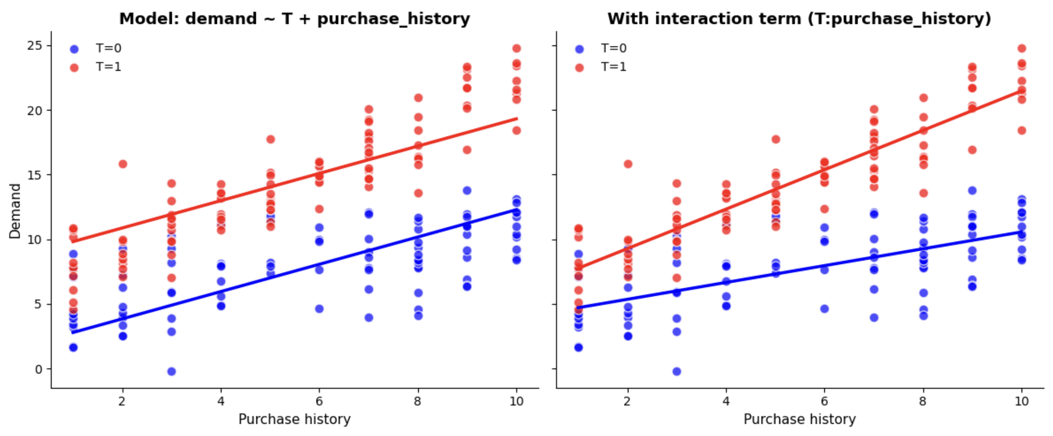
Variables that change the magnitude or direction of the treatment effect across different levels of that variable are called effect modifiers. A surrogate effect modifier is a variable that isn’t a true modifier itself, but is correlated with the true effect modifier, and is used as a proxy. These are used when true effect modifier is unobserved or difficult to measure, for example click behaviour could be a surrogate for a latent trait like motivation. Existing literature or user research can be useful for validating surrogates when you don’t have the data for the modifier.
Evaluation
As mentioned for ATE, there’s no direct test to confirm individual CATE estimates are correct, because we never observe both potential outcomes for any single observation. Individual treatment effects are fundamentally unobservable. However, we can evaluate models of heterogeneity using group-level or out-of-sample checks. The best strategy, when feasible, is to use randomized experimental data for the evaluation. While it may not be possible for model training, running smaller-scale experiments solely for validation is often achievable. Using the randomised treatment, we’re able to get a reliable estimate of the ATE for groups of observations by comparing the treated to the control. Practical approaches for this include:
- Group Average Validation: Divide the sample into bins (e.g. deciles) based on predicted CATE. Then, compare the observed average outcome difference between treatment and control for each group (ATE). If the model captures heterogeneity well, groups with higher predicted CATE should exhibit larger observed treatment effects (i.e. higher sensitivity). If the treatment effect is similar across the groups, then we’re not doing a good job at identifying different sensitivity groups.
- Cumulative Sensitivity Curve: Extending the above, we can compute the cumulative sensitivity as we move from the most to least sensitive observations based on the predicated CATE. When we plot the cumulative sensitivity on Y and the % of the sample on the X (ranked by predicated CATE), we ideally want the curve to start high, and then slowly converge to the ATE (as the CATE of the full sample is just the ATE). For comparison, a random model will just fluctuate around the ATE. This tells us how good is the model’s average prediction by rank.
- Cumulative Gain Curve (uplift): To get something similar to a ROC curve, we can multiply the cumulative sensitivity by the % of the sample used (between 0-1). Multiplying cumulative sensitivity by the % of data used normalizes the cumulative contribution of treatment effect to the overall impact, telling us how much uplift we’ve accumulated so far by targeting the top-ranked individuals. The baseline (random model) will be a straight line from 0 to the ATE, and all models will end at the ATE (as it’s ATE * 1.0). Useful models will show steep curves early on, meaning the highest-ranked individuals benefit most. Flat or erratic curves suggest poor targeting.
- Simulated Decisions: Simulate policy decisions like “treat the top 20% most responsive” and compare the realized lift to random targeting or baseline strategies. This is the same as comparing different cut-offs in the cumulative sensitivity chart, but links heterogeneous effect estimation directly to business outcomes.
- Simulation Studies: Finally, simulation studies using synthetic data where the true CATE is known are another validation approach, mostly used in academic or research settings. These can be helpful during model development to build intuition about estimator behavior under different scenarios, but are generally less applicable in applied settings.
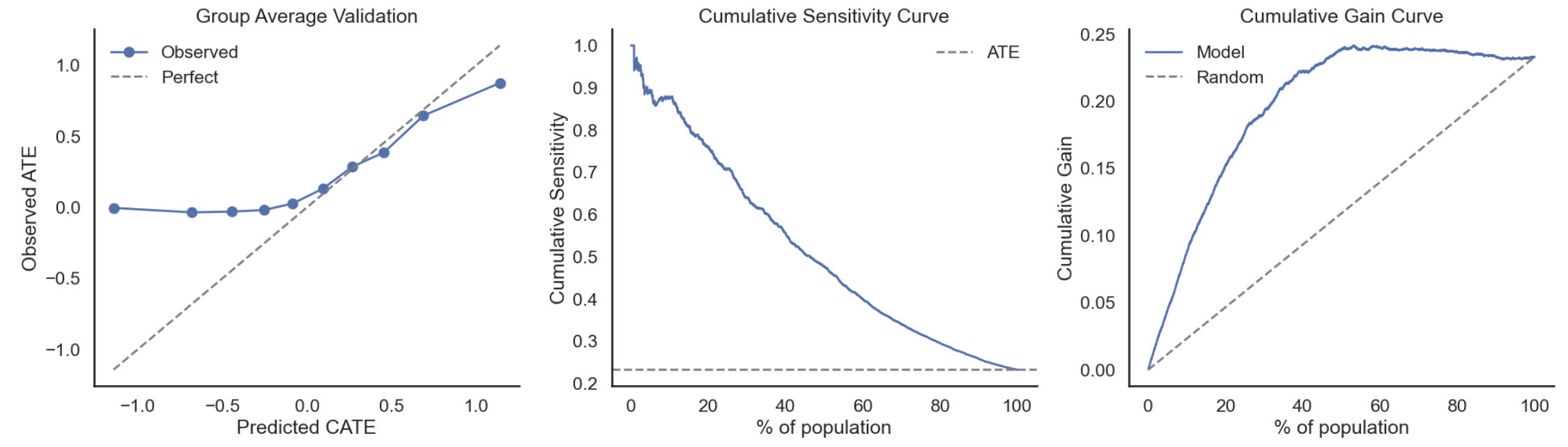 Note: If we use regression to compute the sensitivity, we can also easily add a confidence interval using the standard error
Without randomised data, a common approach is to use cross-validation: train your heterogeneity model on one part of the data, then evaluate how predicted CATEs correspond to observed differences in a holdout set. While this helps us understand whether the results are stable, it doesn’t tell us whether we’re capturing the causal effect (i.e. there can still be bias). Similarly, model performance metrics tell us how well we’re fitting the data. This is useful to avoid overfitting (using cross-validation), but it doesn’t correspond with the accuracy of the causal estimate. For example, a strong \(R^2\) means we’ve fit the data well, but it doesn’t tell us whether we’re capturing the causal relationship of interest (i.e. it could be biased due to confounding).
Ultimately, strong model metrics, good group-level correspondence, and favorable uplift curves based on randomised data provide practical confidence that the heterogeneity model is capturing useful variation for decision-making, even if individual CATEs remain uncertain.
Meta learners
The example above used linear regression to show how we can reframe predictive modeling, not to predict raw outcome values ($Y$), but to predict how the outcome changes with treatment (\(\frac{dY_i}{dT_i}\)). The challenge for applying more flexible or complex machine learning models is that the ground truth isn’t observed for each observation (i.e. we only observe one potential outcome). Yet to apply these models directly, we need to define a target that reflects the Conditional Average Treatment Effect (\(\tau(x)\)) instead of the raw Y values. For binary treatments, one effective solution to this is target transformation (F-learners).
Given:
- Binary treatment \(T_i \in \{0,1\}\)
- Outcome \(Y_i\)
- Treatment assignment probability \(p = \mathbb{E}[T]\) (e.g. 50% in a randomised trial)
- \(\tau(x)\) = Conditional Average Treatment Effect (CATE)
We define the transformed outcome as:
\[\tilde{Y}_i = \frac{Y_i - \bar{Y}}{p(1 - p)} \cdot (T_i - p)\]With random assignment (or unconfoundedness), this transformation satisfies:
\[\mathbb{E}[\tilde{Y} \mid X = x] = \tau(x)\]This allows us to train any regression or machine learning model to predict \(\tilde{Y}_i\), and the model’s predictions will approximate \(\tau(x)\), the individual-level treatment effect. This approach is called an F-learner, where you transform the outcome and then fit a model to predict it. However, the transformed outcome $$\tilde{Y}_i$ $is often noisy, especially when treatment assignment is highly imbalanced. Therefore, this method works best with large datasets where noise averages out.
This is just one example of a meta learner for CATE estimation, with “meta” refering to the fact they wrap around standard supervised learning models to estimate CATE.
| Learner | What it Estimates | Models Fit | Formula for CATE \(\hat{\tau}(x)\) | Pros | Cons |
|---|---|---|---|---|---|
| S-learner | \(\mathbb{E}[Y \mid X, T]\) | Single model \(\hat{f}(X, T)\) (fit model predicting \(Y\) using \(X\) and \(T\) as features) | \(\hat{\tau}(x) = \hat{f}(x, 1) - \hat{f}(x, 0)\) | Simple; works with any supervised ML model | Can underfit heterogeneity, especially if regularization shrinks or drops \(T\) coefficient |
| T-learner | \(\mathbb{E}[Y \mid X=x, T=1]\) and \(\mathbb{E}[Y \mid X=x, T=0]\) | Two models: \(\hat{\mu}_1(x) = \mathbb{E}[Y \mid X=x, T=1]\) and \(\hat{\mu}_0(x) = \mathbb{E}[Y \mid X=x, T=0]\) | \(\hat{\tau}(x) = \hat{\mu}_1(x) - \hat{\mu}_0(x)\) | Flexible; allows different complexity for treatment/control groups | Needs sufficient \(n\) in both groups; imbalance can distort differences |
| X-learner | Weighted combination of imputed individual treatment effects | 1. Fit \(\hat{\mu}_1(x), \hat{\mu}_0(x)\) as in T-learner 2. Impute: \(D_1 = Y - \hat{\mu}_0(x), \quad D_0 = \hat{\mu}_1(x) - Y\) 3. Fit \(g_1(x), g_0(x)\) to imputed ITEs 4. Estimate \(e(x) = P(T=1 \mid X=x)\) |
\(\hat{\tau}(x) = e(x) \cdot g_0(x) + (1 - e(x)) \cdot g_1(x)\) | Handles imbalance well; leverages both groups | Requires multiple models; sensitive to propensity or outcome model misspecification |
| F-learner | \(\mathbb{E}[\tilde{Y} \mid X = x]\), with transformed outcome \(\tilde{Y}\) | Model \(\hat{g}(x) \approx \mathbb{E}[\tilde{Y} \mid X = x]\), where \(\tilde{Y} = \frac{Y - \bar{Y}}{p(1-p)}(T - p), \quad p = P(T=1)\) | \(\hat{\tau}(x) = \hat{g}(x)\) | Works with any ML model on transformed \(\tilde{Y}\) | High variance; works better with large datasets |
| R-learner | Orthogonalized residual treatment effect | 1. Estimate: \(\hat{m}(x) = \mathbb{E}[Y \mid X=x]\), \(\hat{e}(x) = P(T=1 \mid X=x)\) 2. Minimize: \(\sum_i ( (Y_i - \hat{m}(X_i)) - (T_i - \hat{e}(X_i)) g(X_i) )^2\) |
\(\hat{\tau}(x) = \hat{g}(x)\) | Reduces bias from nuisance parameters; integrates well with orthogonalization and DML | Requires reliable nuisance models; more computationally intensive |
Causal Forests
Causal forests are a nonparametric method for estimating heterogeneous treatment effects. They extend random forests to the causal inference setting, using modified tree-splitting rules that are sensitive to treatment effect variation to estimate CATE.
The algorithm proceeds in two main phases:
-
Honest splitting: The data is randomly divided into two subsets. One subset is used to build trees (i.e. decide how to split), and the other is used to estimate treatment effects within each leaf. This prevents overfitting and enables valid inference.
-
Splitting criterion: Instead of minimizing prediction error (as in standard regression trees), splits are chosen to maximize heterogeneity in treatment effects between child nodes. This focuses the model on capturing meaningful variation in treatment response.
Each tree estimates local treatment effects in its leaves, and the forest averages these estimates to produce a smooth CATE function $\hat{\tau}(x)$.
Causal forests make minimal parametric assumptions and can flexibly handle complex interactions and nonlinearities. They also support valid variance estimates for CATEs, enabling hypothesis testing and confidence intervals at the individual or group level.
BART (Bayesian Additive Regression Trees)
BART is a Bayesian nonparametric method that models complex functions by summing across many shallow regression trees. For causal inference, BART is typically applied to estimate potential outcomes $\hat{Y}(1)$ and $\hat{Y}(0)$ separately, allowing the CATE to be computed as their difference.
Key features of BART for CATE estimation:
- Modeling flexibility: BART can capture nonlinearities and high-order interactions without explicit feature engineering.
- Posterior uncertainty: Since BART is Bayesian, it produces full posterior distributions over predicted outcomes and treatment effects, which you can use to quantify uncertainty in CATE estimates.
- No need for propensity modeling: When used with unconfounded data, BART can be directly applied to estimate counterfactuals. However, in practice, it is often paired with propensity score weighting or used in doubly robust frameworks for added stability.
| A typical BART setup for causal inference models $Y \sim f(X, T)$, allowing the treatment effect to vary with covariates. Alternatively, you can estimate $f_1(X) = E[Y | T=1, X]$ and $f_0(X) = E[Y | T=0, X]$ separately, then take $\hat{\tau}(X) = f_1(X) - f_0(X)$. |
BART is particularly strong when you care about uncertainty-aware estimates or want a smooth, nonparametric model of individual treatment effects.
Representation learning methods (TARNet / CFRNet / DragonNet)
Representation learning methods for CATE estimation use neural networks to learn a shared feature representation that captures relevant structure in the covariates before estimating potential outcomes. The goal is to improve generalization by balancing treated and control groups in a learned latent space, especially in the presence of covariate shift.
TARNet (Treatment-Agnostic Representation Network) is the baseline architecture: it first passes covariates through a shared representation network and then branches into two outcome heads—one for treated and one for control units.
CFRNet (Counterfactual Regression Network) builds on TARNet by adding a regularization term (typically based on Integral Probability Metrics like MMD or Wasserstein distance) that explicitly encourages the learned representation to balance the distribution of treated and control units.
DragonNet extends this further by jointly predicting the propensity score within the network and incorporating a targeted regularization loss to improve bias correction and efficiency.
These methods are flexible and can model complex, non-linear treatment effect heterogeneity. However, they typically require large amounts of training data and careful hyperparameter tuning. Because of their black-box nature, interpretability is limited compared to tree-based models. Despite these challenges, representation learning approaches have become popular for personalized intervention tasks and counterfactual prediction when large observational datasets are available.
Comparison
| Method | How It Works | Data Needed | Key Strengths | Key Limitations |
|---|---|---|---|---|
| Meta-Learners (S-, T-, X-, F-) | Use standard ML models in structured ways to estimate treatment effects, e.g., separate models per group or using transformed targets. | Cross-sectional | Modular; can plug in any ML model; widely used and understood. | Susceptible to overfitting; no built-in uncertainty quantification. |
| R-Learner | Residualizes both outcome and treatment, then regresses the residuals to estimate treatment effects. | Cross-sectional | Orthogonalization reduces bias; compatible with flexible models. | Sensitive to errors in nuisance models; more complex than meta-learners. |
| Causal Forests (GRF) | Builds tree-based ensemble models that split to maximize treatment effect heterogeneity using “honest” sample splitting. | Cross-sectional or panel | Captures non-linear, non-additive heterogeneity; includes uncertainty estimates. | Less interpretable; slower training; may require large samples. |
| BART (Bayesian Additive Regression Trees) | Bayesian ensemble of trees modeling both outcomes and treatment heterogeneity, with posterior uncertainty. | Cross-sectional or panel | Provides full posterior over effects; robust to model misspecification. | Computationally intensive; harder to scale to very large datasets. |
| Representation Learning (TARNet / CFRNet / DragonNet) | Use deep neural networks to learn shared representations of covariates before modeling treatment-specific outcomes. CFRNet adds balancing loss; DragonNet also predicts propensity scores. | Cross-sectional (large N) | Flexible architectures; balance improves generalization; end-to-end training. | Requires large training data; tuning is complex; lower interpretability. |
| GANITE | Uses Generative Adversarial Networks to model counterfactual outcomes directly, via adversarial training. | Cross-sectional (large N) | Can explicitly generate counterfactuals; models complex data distributions. | Hard to train and tune; interpretability is low; GANs require care to avoid mode collapse. |
General CATE estimation challenges
Estimating heterogeneous treatment effects (CATE) is essential for personalization and targeting, but it is substantially harder and noisier than estimating overall average treatment effects (ATE). The fundamental difficulty is that we only observe one outcome for each individual. This means CATE is estimated in expectation over groups of individuals with similar covariates, not at the individual level.
Several challenges follow:
- Small sample sizes within groups: As we condition on more features (high-dimensional covariates), the number of individuals sharing the same covariates shrinks, making estimates noisier.
- Uneven treatment assignment: If some subgroups receive more or less treatment, naive comparisons can mistake differences due to treatment range or assignment imbalance for real effect heterogeneity.
- Non-linear relationships: Effect heterogeneity may not come from true differences in how groups respond, but instead from non-linear transformations of either the treatment or the outcome. This is especially problematic with binary outcomes, but can also affect continuous treatments.
The issues with binary outcomes are not specific to CATE (as covered earlier), but their impact is more pronounced when estimating heterogeneous effects. For ATE, the averaging helps smooth out variance and nonlinearities to some extent. For CATE, the nonlinearity, baseline dependence, and variance can distort effect estimates and create false signals of heterogeneity.
Focusing on Decisions, Not Just Estimates
Fortunately, we usually do not need precise individual-level CATE estimates. In practice, we want good decisions about who to prioritize. Several strategies help shift focus from noisy point estimates to decision-relevant metrics:
- Uplift curves (or gain charts): Plot the cumulative benefit as you target increasing proportions of the population, ranked by predicted uplift. Useful for choosing how much of your population to target.
- Ranking scores: Often, ordering individuals by expected benefit matters more than the exact magnitude of their estimated CATE. For example, targeting the top \(10\%\) most responsive customers.
- Binned or aggregated estimates: By grouping individuals into bins (for example, deciles of predicted uplift), you can reduce variance and provide more stable, interpretable summaries of treatment effects. This is often closer to how targeting decisions are actually made at scale.
By emphasizing stable rankings and group-level effects over noisy individual estimates, you can still make effective personalized decisions even when CATE estimates are imperfect.
Longitudinal Methods
In many applied settings, data are collected repeatedly over time for the same individuals or units, creating longitudinal datasets. Analyzing longitudinal data introduces unique challenges such as time-varying confounding, informative loss to follow-up, and complex outcome structures like time-to-event data. Addressing these issues requires specialized methods that properly account for the evolving relationships between treatments, covariates, and outcomes over time. In this section, we review key longitudinal causal methods designed to handle these challenges.
Time-Varying Confounding
In many real-world settings, both treatments and confounders change over time. A user’s health status, engagement level, or behavior might influence future treatment, and also future outcomes. This creates a feedback loop where past treatment affects future confounders, which in turn affect subsequent treatment. If you’re goal is to measure the cumulative effect of treatment (e.g. the effect of repeated notifications), then specialised methods are necessary.
For example, suppose you’re interested in whether mobile notifications increase weekly user engagement (e.g. minutes of app use, or days active). You observe users across multiple weeks, and each week they may or may not receive a push notification. However, users who were less engaged in the prior week are more likely to be targeted for a notification in the current week. At the same time, past engagement is predictive of current engagement. This makes prior engagement a time-varying confounder: it affects both the treatment (notifications) and the outcome (future engagement), but is itself influenced by earlier treatment. Naively adjusting for a time-varying confounder in a static model can block part of the treatment effect or introduce collider bias, leading to biased estimates. This is similar to the issue of controlling for post treatment variables with a single treatment, but in longitudinal settings with repeated treatments, this issue becomes more complex and common, generally requiring specialized methods.
Simplication: single treatment point
Starting with the simplest option first, in some cases you can mitigate time-varying confounding by selecting a single treatment time point per user. Using the notifications example:
- You define a “baseline period” (e.g., week 0).
- You define treatment as: receiving a notification in week 1.
- You define outcome as: engagement in week 2 or later.
- You only condition on baseline covariates (including engagement in week 0), which are not affected by treatment.
This setup lets you approximate a static causal effect, avoiding the key pitfall of time-varying confounding, namely, that your confounder is influenced by prior treatment. However, there are a number of limitations:
- You’re throwing away a lot of data (all but one treatment opportunity per user).
- You’re not estimating the effect of repeated or sustained treatment, just the effect of one notification at one point in time.
- If users are selected into treatment based on earlier behavior (e.g. the notification decision still depends on things before the baseline period like demographics or signup behaviour), even the first observed treatment may still be confounded (i.e. the baseline is too late).
- Even within the baseline (e.g. week 0), you still need to correctly measure and adjust for all confounders of the treatment (notification in week 1) and the outcome (engagement in week 2+).
If you’re okay estimating the effect of a one-time treatment, and can clearly define pre-treatment covariates, then selecting a single point may be a reasonable simplification.
G-methods
If your goal is to estimate the cumulative or dynamic effect of repeated treatments (e.g. the effect of receiving multiple notifications over time), then you can’t just control for all covariates at the final time step, or even at each step, without risking bias. G-methods methods can account for the feedback loops that occur when prior treatment influences future covariates, which in turn affect subsequent treatment and outcomes (i.e. time varying confounding). Common G-methods for longitudinal problems include: G-computation (or the G-formula), Inverse Probability Weighting (IPW), and Marginal Structural Models (MSMs).
All of these require aligning treatment, covariate, and outcome data longitudinally, and they rely on the same core assumptions: positivity, consistency, and sequential exchangeability (no unmeasured confounding at each time).
Before applying any of these, you’ll need to:
- Transform your data into long format, one row per user per time unit (e.g. week).
- Define your treatment \(A_t\), covariates \(L_t\), and outcome Y (usually measured at the end) at each time step.
- Ensure covariates used to adjust for confounding are measured prior to treatment at that step.
G-computation (or the G-formula)
As in the static case, G-computation estimates causal effects by explicitly modeling outcomes under different treatment regimes. However, in longitudinal settings, we simulate sequences of outcomes over time. G-computation avoids conditioning on post-treatment variables directly by simulating what would happen under full treatment strategies (e.g. “always treat,” “never treat,” or “treat only if inactive last week”).
The key idea is:
-
Model the outcome at each time step as a function of past treatment and covariate history:
\[E[Y_t \mid A_{0:t}, L_{0:t}]\] -
Model covariate evolution (if needed): If covariates are affected by past treatment, model them too:
\[P(L_t \mid A_{0:t-1}, L_{0:t-1})\] -
Simulate counterfactual outcomes under hypothetical treatment strategies: For each user, simulate forward from baseline to generate treatment, covariate, and outcome paths consistent with a given policy:
-
At each time step:
- Set treatment $A_t$ based on the strategy
- Predict $L_t$ using the covariate model (if applicable)
- Predict $Y_t$ using the outcome model
-
-
Average outcomes across users to estimate the causal effect of each strategy:
\[\hat{E}[Y^{\bar{a}}] = \frac{1}{n} \sum_{i=1}^{n} \hat{Y}_i^{\bar{a}}\]
Example
Suppose you want to estimate the effect of sending a notification each week for two weeks on engagement in week 3. Each user has:
- $L_0$: Initial engagement (active or inactive)
- $A_1$: Notification in week 1 (binary)
- $L_1$: Engagement in week 1 (time-varying covariate)
- $A_2$: Notification in week 2 (binary)
- $Y$: Engagement in week 3 (final outcome)
We do not model engagement in week 2 because we assume the final outcome $Y$ depends only on prior engagement and treatment, not directly on engagement in week 2. This simplifies simulation by removing the need to predict $L_2$.
Steps:
-
Fit the outcome model:
Model $Y$ as a function of $[L_0, A_1, L_1, A_2]$ (e.g., logistic regression). This allows you to simulate $Y$ under any counterfactual history. -
Fit the covariate model:
Model $L_1$ as a function of $[L_0, A_1]$ (e.g., logistic regression). This allows you to simulate week 1 engagement under different treatments. -
Simulate outcomes for each user and treatment strategy:
- Always-treat strategy ($A_1 = 1$, $A_2 = 1$):
- Set $A_1 = 1$
- Predict $\hat{L}_1 \sim P(L_1 \mid L_0, A_1 = 1)$
- Set $A_2 = 1$
- Predict $\hat{Y} \sim P(Y \mid L_0, A_1 = 1, \hat{L}_1, A_2 = 1)$
- Never-treat strategy ($A_1 = 0$, $A_2 = 0$):
Repeat the steps above with $A_1 = 0$ and $A_2 = 0$
Optionally, repeat the simulation multiple times per user and average the results to reduce randomness from sampling.
- Always-treat strategy ($A_1 = 1$, $A_2 = 1$):
-
Estimate causal effects:
\[\hat{E}[Y \mid \text{always treat}] - \hat{E}[Y \mid \text{never treat}]\]
Average predicted $Y$ across users for each strategy. Then take the difference:
Note, we do not model how treatment was originally assigned (e.g. whether $A_1$ depends on $L_0$, which it very well may). Instead, we explicitly set treatment values according to predefined strategies, overriding the observed treatment. This means we do not require $A_1$ to be independent of baseline covariates like $L_0$.
However, the example above assumes that the treatment strategy is fixed in advance (e.g. always treat or never treat). In practice, treatment decisions are often dynamic (based on user behavior). For instance, you might send a notification in week 2 only if the user was inactive in week 1. In such cases, treatment depends on simulated covariates like $\hat{L}_1$, and the simulation must be adapted to reflect that dependency.
When treatment depends on simulated covariates
If your treatment rule depends on user behavior, and user behavior depends on past treatment, then you can’t simulate one without the other. You must recursively simulate covariates and then use them to apply your treatment rule at each time step. For example:
Suppose your strategy is: “notify in week 2 only if the user was inactive in week 1.”
You must simulate the user’s week 1 engagement before you can assign treatment in week 2.
Steps:
- Start from baseline $L_0$ and assign $A_1$
- Predict $\hat{L}_1 \sim P(L_1 \mid L_0, A_1)$
- Apply policy: if $\hat{L}_1 = 0$ (inactive), then set $A_2 = 1$; else $A_2 = 0$
- Use $[L_0, A_1, \hat{L}_1, A_2]$ to predict $Y$
Repeat this process for each user. Then average predicted outcomes to estimate effects under this policy. Compare against other strategies as before.
When the outcome spans multiple time points
If your outcome is measured over time (e.g., weekly engagement from week 1 to week 4), then you must simulate the outcome recursively at each time step. Each prediction depends on the full simulated treatment and covariate history up to that point. For example, suppose your outcome is engagement in weeks 1–3, and you want to simulate the effect of sending notifications each week. You must predict $Y_1$, $Y_2$, and $Y_3$ in sequence, conditioning each on the relevant treatment and covariates observed so far.
Steps:
- Start from baseline covariates $L_0$
- Assign $A_1$ (e.g. always treat)
- Predict $\hat{L}_1 \sim P(L_1 \mid L_0, A_1)$
- Predict $\hat{Y}_1 \sim P(Y_1 \mid L_0, A_1, \hat{L}_1)$
- Assign $A_2$ based on your strategy (e.g., always treat or policy rule)
- Predict $\hat{L}_2 \sim P(L_2 \mid \hat{L}_1, A_2)$
- Predict $\hat{Y}_2 \sim P(Y_2 \mid \hat{L}_1, A_2, \hat{L}_2, \hat{Y}_1)$
- Repeat for $A_3$, $\hat{L}_3$, and $\hat{Y}_3$
At the end, you’ll have a full simulated outcome trajectory under each treatment strategy:
$[\hat{Y}_1, \hat{Y}_2, \hat{Y}_3]$
You can then define your final outcome as: a specific time point (e.g. $\hat{Y}_3$); a cumulative measure (e.g. total weeks engaged: $\hat{Y}_1 + \hat{Y}_2 + \hat{Y}_3$); or, a binary indicator (e.g. ever engaged). Some more examples below linking it to the question:
| Causal Question | Final Estimate |
|---|---|
| What’s the effect of always treating on engagement in week 8? | $\hat{E}[Y_8^{\bar{a}}]$ |
| What’s the effect of always treating on total engagement over 8 weeks? | $\hat{E}\left[\sum_{t=1}^8 Y_t^{\bar{a}}\right]$ |
| What’s the effect on probability of engaging in any week? | $\hat{E}\left[\mathbb{I}\left(\max_t Y_t^{\bar{a}} = 1\right)\right]$ |
| What’s the effect on number of active weeks? | $\hat{E}\left[\sum_t \mathbb{I}(Y_t = 1)\right]$ |
| What’s the probability of being engaged in every week? | $\hat{E}\left[\mathbb{I}(Y_1 = 1 \land \dots \land Y_8 = 1)\right]$ |
Repeat the simulation across users and strategies, then compare average outcomes as before.
Model choice
As in the static case, this approach is more of a framework. Any predictive model that can estimate the conditional expectation of the outcome and time-varying covariates can be used. Logistic regression is a standard choice when the outcome is binary, and linear regression is often used for continuous outcomes. However, more flexible models such as random forests, gradient boosting, or neural networks can also be used, especially when you expect non-linear relationships or complex interactions. The key requirement is that the models are well-calibrated and accurately capture the conditional distributions needed for simulating counterfactual outcomes.
Estimating Uncertainty
Since G-computation involves multiple modeled steps and stochastic simulations, it’s good practice to use bootstrapping and nested simulations to estimate confidence intervals and capture both model and simulation uncertainty.
-
Point estimate: Fit all models on the original dataset. For each user and strategy, run multiple simulations and average the simulated outcomes to get a stable point estimate (reducing randomness from stochastic predictions).
- Bootstrapping to get CIs: Resample users with replacement and refit all models on each bootstrap sample. Within each bootstrap iteration:
- Optionally, run multiple simulations per user and average to reduce noise
- Estimate the treatment effect
- Combine to get CIs: After all iterations, collect the estimated effects to form an empirical distribution
- Use percentiles (e.g. 2.5th, 97.5th) or compute standard error and apply normal approximation (e.g. $\hat{\tau} \pm 1.96 \times \text{SE}$).
- Efficiency tip: For the main point estimate, use many simulations per user for stability. In bootstrapping, using fewer simulations (even 1 per user) can save compute, at a slight cost to precision
IPW (Inverse Probability Weighting)
Inverse Probability Weighting (IPW) is an alternative to G-computation for handling time-varying confounding in longitudinal data. The core idea is to create a pseudo-population in which treatment assignment at each time point is independent of measured confounders. This allows for unbiased estimation of causal effects by effectively balancing the treated and untreated groups over time. IPW relies on the assumptions of positivity (every individual has a nonzero probability of receiving each treatment level at each time), consistency, and sequential exchangeability (no unmeasured confounding at each time step). Correctly specifying the treatment assignment models (propensity scores) is crucial for valid inference.
How it works in time-varying settings:
-
At each time step $t$, estimate the probability of receiving the treatment actually observed, conditional on the full history of past treatments and covariates up to time $t$. This is the estimated propensity score, where $L_{0:t}$ are covariates and $A_{0:t-1}$ are prior treatments:
\[P(A_t = a_t \mid L_{0:t}, A_{0:t-1})\] -
Calculate weights for each individual by taking the inverse of the product of these conditional probabilities across all time points:
\[w_i = \prod_{t=1}^T \frac{1}{P(A_t = a_t \mid L_{0:t}, A_{0:t-1})}\] -
To improve stability, stabilized weights are often used, which replace the numerator with the marginal probability of treatment:
\[w_i^{\text{stab}} = \prod_{t=1}^T \frac{P(A_t = a_t)}{P(A_t = a_t \mid L_{0:t}, A_{0:t-1})}\] -
These weights reweight the sample to create a pseudo-population where treatment is randomized with respect to observed confounders, effectively removing confounding bias.
-
After computing weights, fit a weighted regression model for the outcome on treatment history, without adjusting for confounders (because confounding is accounted for by the weights). The choice of regression model (e.g., linear, logistic) determines the interpretation of coefficients and must be chosen according to the outcome type and desired estimand.
Example
Suppose you want to estimate the effect of sending push notifications each week on user engagement. Each user is observed over multiple weeks, with variables:
- $L_0$: Baseline engagement (binary: active or not)
- $A_1$: Notification in week 1 (binary)
- $L_1$: Engagement in week 1
- $A_2$: Notification in week 2
- $L_2$: Engagement in week 2
- … and so forth.
At each week $t$, users may receive a notification based on their prior engagement and notification history (time-varying confounding). For example, less engaged users might be more likely to receive notifications. We want to estimate the causal effect of $A_1$ and $A_2$ on engagement in week 3, adjusting for time-varying confounding.
Steps:
-
Estimate propensity scores for each week: For binary treatments, this is typically done using logistic regression.
For week 1, model:
\[P(A_1 = a_1 \mid L_0)\]For week 2, model:
\[P(A_2 = a_2 \mid L_0, A_1, L_1)\]And similarly for later weeks.
-
Calculate stabilized weights:
For each user, the weight up to week 2 is:
\[w_i = \frac{P(A_1 = a_1) \times P(A_2 = a_2)}{P(A_1 = a_1 \mid L_0) \times P(A_2 = a_2 \mid L_0, A_1, L_1)}\]This downweights users with unlikely treatment histories conditional on their covariates, balancing the treated and untreated groups.
-
Fit weighted outcome model:
Fit a weighted regression of week 3 engagement $Y$ on treatment history $A_1, A_2$, without adjusting for covariates because the weights account for confounding.
\[E[Y \mid A_1, A_2]\]Typical choices include:
- Linear probability model: coefficients interpreted as average differences in probability (percentage points).
- Logistic regression: coefficients interpreted as log-odds ratios (less intuitive but suitable for binary outcomes).
-
Interpret results:
The coefficients on $A_1$ and $A_2$ estimate the marginal causal effect of receiving notifications in weeks 1 and 2 on engagement in week 3, averaged over the population. For example, if the coefficient for $A_2$ in a linear model was 0.15, we could say: “receiving a notification in week 2 increases the probability of engagement in week 3 by 15 percentage points, on average.” The total effect of receiving notifications in both weeks is the sum of the coefficients (under a linear model assumption).
This differs from G-computation, which estimates conditional expectations and uses simulation; IPW estimates the marginal effect by reweighting the observed data.
-
Quantify uncertainty:
Because the weights and outcome model are both estimated, standard errors should reflect uncertainty in both steps. A common approach is bootstrapping:
- Resample the data with replacement many times (e.g., 500–1000 iterations).
- For each bootstrap sample:
- Re-estimate propensity score models and stabilized weights.
- Refit the weighted outcome model.
- Record treatment effect estimates (e.g., coefficients or contrasts).
- Use the empirical distribution of estimates to compute confidence intervals (e.g., percentile-based or normal approximation).
Practical considerations
-
IPW estimates can be unstable if some individuals have very low probabilities of receiving their observed treatment, leading to extreme weights that inflate variance and bias. To address this:
- Examine the weight distribution (histograms, summary stats).
- Consider truncating or trimming weights at a threshold.
- Use stabilized weights to improve variance properties.
- Correct model specification for propensity scores is essential; misspecification leads to biased weights and causal estimates.
- IPW naturally extends to longer time horizons and complex dynamic treatment rules by including the relevant treatment and covariate history in the propensity models.
- IPW can be combined with outcome modeling (e.g., augmented IPW, doubly robust estimators) to improve efficiency and robustness.
IPW weights can also be used to estimate treatment effects on outcomes measured at multiple time points by fitting weighted models for each outcome, or the full outcome trajectory. However, to explicitly model the effect of treatment histories on longitudinal outcomes, Marginal Structural Models (MSMs) are typically employed.
Marginal Structural Models (MSMs)
Marginal Structural Models (MSMs) provide a framework for estimating the causal effects of dynamic treatment strategies in the presence of time-varying confounding. Like IPW and G-computation, MSMs aim to recover causal effects from observational data, but they go a step further by explicitly modeling how treatment history influences outcomes over time. The key idea behind an MSM is to model the marginal, or population-average, relationship between treatment and outcome. This is typically done using a generalized linear model (GLM), such as linear regression for continuous outcomes or logistic regression for binary outcomes. These models yield coefficients that can be interpreted as average treatment effects across the population. Typically, IPW is implemented first to reweight the data, creating a pseudo-population in which treatment assignment is independent of past covariates. The MSM is then fit to this weighted data to estimate causal effects. This combination of reweighting followed by outcome modeling distinguishes MSMs from IPW alone and allows them to handle complex longitudinal treatment patterns without conditioning directly on post-treatment variables.
Example with a single final outcome:
Suppose you want to understand the effect of receiving weekly notifications on user engagement measured at week 3. The data includes:
- $L_0$: Baseline engagement
- $A_1, A_2$: Notifications received in weeks 1 and 2 (binary indicators)
- $L_1, L_2$: Engagement measured weekly (time-varying confounders)
- $Y$: Engagement at week 3 (outcome)
Users may be more likely to receive notifications if they showed low engagement in previous weeks, creating time-varying confounding.
Steps:
-
Estimate stabilized inverse probability weights (IPW):
For each week $t$, estimate the probability of receiving the observed treatment $A_t$ conditional on past covariates and treatments. These are typically modeled with logistic regression:
\[P(A_t = a_t \mid L_0, A_1, L_1, \dots, A_{t-1}, L_{t-1})\]Then compute stabilized weights as the product of marginal treatment probabilities divided by these conditional probabilities:
\[w_i^{\text{stab}} = \prod_{t=1}^2 \frac{P(A_t = a_t)}{P(A_t = a_t \mid L_0, A_1, L_1, \dots, A_{t-1}, L_{t-1})}\]Note: Check for extreme weights and consider truncation or smoothing to improve stability.
-
Specify the MSM:
Choose a parametric model relating the expected potential outcome $Y^{\bar{a}}$ to treatment history. For example:
\[E[Y^{\bar{a}}] = \beta_0 + \beta_1 A_1 + \beta_2 A_2 + \beta_3 \text{(baseline covariates)}\] -
Fit the MSM using weighted regression:
Fit the model for $Y$ on treatment history variables using the stabilized IP weights, without including time-varying confounders as covariates. This weighted regression estimates marginal causal effects averaged over confounders.
-
Interpret coefficients:
In this context, marginal effects refer to population-average causal effects. Rather than measuring the effect conditional on specific covariate values (as in traditional regression), MSMs estimate the average effect of treatment history across the entire study population, after balancing confounders via weighting. This means the effects describe how the average outcome would change if everyone in the population received a particular treatment pattern, marginalizing over differences in covariates.
- $\beta_1$ estimates the average causal effect of receiving a notification in week 1 on engagement at week 3.
- $\beta_2$ estimates the average causal effect of receiving a notification in week 2 on engagement at week 3.
MSMs with multiple outcome time points
When outcomes are measured repeatedly over time (e.g., weekly engagement from week 1 to week 3 or beyond), MSMs can be extended to model the entire outcome trajectory as a function of treatment history.
For example, suppose you observe engagement outcomes $Y_1, Y_2, Y_3$ and want to estimate how notifications in weeks 1 and 2 affect engagement over this period.
-
Compute stabilized IP weights as before, based on treatment and covariate histories.
-
Specify an MSM modeling the marginal mean outcome at each time point $t$:
\[E[Y_t^{\bar{a}}] = \beta_0 + \beta_1 A_1 + \beta_2 A_2 + \beta_3 t + \beta_4 (A_1 \times t) + \beta_5 (A_2 \times t) + \beta_6 \text{(baseline covariates)}\]This specification allows treatment effects to vary over time.
-
Fit this model using weighted regression or generalized estimating equations (GEE) to account for within-subject correlation, applying the IP weights.
-
Interpret coefficients as the average causal effect of treatment history on the trajectory of engagement over time.
Practical Considerations:
- Weight diagnostics: Since MSMs rely heavily on IP weights, it’s essential to inspect the distribution of weights for instability. Large or extreme weights can make estimates sensitive to a small number of observations and increase variance. Common strategies include weight truncation (e.g. capping weights at the 1st and 99th percentiles) or using stabilized weights to reduce variability.
- Model selection and interactions: Because MSMs allow for flexible outcome models, it’s important to consider whether treatment effects may vary over time or interact with baseline covariates. Including time-by-treatment interactions, for example, can help capture changes in effectiveness across the study period.
- Choice of functional form: Although MSMs are often implemented as linear or logistic regressions, more flexible forms can be used when appropriate, including polynomial terms or splines. However, more complex models increase the risk of overfitting, particularly with limited sample size or rare treatment histories.
MSMs fill an important niche between fully conditional approaches like G-computation and non-parametric weighting approaches like IPW. By explicitly modeling outcomes while using weighting to balance confounders, they offer a blend of flexibility and interpretability.
Method comparison
| Aspect | Simplification: Single Treatment Point | G-computation (G-formula) | IPW (Inverse Probability Weighting) | MSMs (Marginal Structural Models) |
|---|---|---|---|---|
| Method Overview & Modeling Approach | Uses standard regression to estimate treatment effect at one fixed time point, conditioning only on baseline covariates. No modeling of treatment assignment or covariate evolution. | Sequential modeling of outcomes and covariates over time, simulating full treatment and covariate trajectories under different treatment strategies. Requires correctly specified outcome and covariate models. | Models treatment assignment probabilities (propensity scores) at each time point to calculate weights that create a pseudo-population with balanced confounders; no outcome model needed for weighting. | Combines IP weights with a weighted regression model of outcome on treatment history, estimating marginal treatment effects averaged over the population without conditioning on confounders directly. |
| Estimand & Interpretation | Conditional effect of a one-time treatment at a specific time, given baseline covariates. | Conditional expected outcomes under specified dynamic treatment strategies, accounting for treatment-confounder feedback. | Marginal (population-average) causal effect of treatment history, reflecting average effect across the population. | Marginal (population-average) treatment effects capturing how treatment history affects outcomes on average over the population, can include time-varying effects. |
| Handling Time-varying Confounders | Avoids time-varying confounding by only adjusting for baseline covariates; ignores repeated treatments and their feedback. | Explicitly models time-varying confounders and their evolution, simulating their interaction with treatment over time. | Adjusts for time-varying confounders indirectly by weighting observations according to inverse probability of observed treatment history given covariates. | Same as IPW, with the addition of outcome modeling to capture treatment effect marginally; weights balance confounders before outcome regression. |
| Assumptions | No unmeasured confounding at baseline; treatment assignment at the chosen time is independent of unmeasured factors given baseline covariates. | Positivity, consistency, sequential exchangeability; correct model specification for both covariate and outcome processes. | Positivity, consistency, sequential exchangeability; correct specification of treatment assignment (propensity) models at all times. | Same as IPW, plus correct specification of MSM outcome model; relies on stable weights for reliable estimates. |
| Strengths | Simple and easy to implement; interpretable; requires fewer assumptions; suitable for short-term or single treatment effect questions. | Highly flexible; can evaluate complex, dynamic treatment regimes with feedback; allows direct simulation of counterfactual outcomes. | Conceptually straightforward; avoids outcome modeling bias; targets marginal causal effects; scalable to longer time horizons. | Balances confounding with weights and incorporates outcome regression for efficiency; interpretable marginal effects; flexible for dynamic treatments and repeated outcomes. |
| Limitations | Discards information on repeated treatments; may suffer residual confounding if baseline covariates are incomplete; not suitable for cumulative or dynamic effects. | Computationally intensive; sensitive to misspecification of multiple models; simulation can be complex and resource-heavy. | Sensitive to extreme or unstable weights; requires careful model checking and diagnostics; no direct outcome modeling may limit efficiency. | Shares weighting challenges with IPW; outcome model must be correctly specified; can be unstable with complex or sparse data; requires balance between flexibility and complexity. |
| Recommended Use Cases | Short time horizon; interest in a single treatment effect; when only baseline covariates are reliable; simpler scenarios. | Evaluating specific static or dynamic treatment rules involving time-varying confounding and feedback loops; when flexible outcome modeling is feasible. | Estimating marginal population-level effects over longer time horizons; when avoiding outcome model bias is important; computational tractability preferred. | When population-average causal effects are desired with complex treatment histories; balancing interpretability with flexibility; often preferred for longer or repeated outcome data. |
Dropout (loss to follow-up)
In longitudinal studies and real-world observational settings, it’s common for some users or subjects to stop providing data before the study ends. This is called loss to follow-up or dropout. If dropout is related to both the treatment and the outcome, it can bias your estimates. For example, if users who disengage differ systematically from those who stay, treating the missing data as random will lead to distorted results. This is known as informative censoring, because the missingness carries information about the outcome.
Ignoring it
Before applying specialized methods, it’s worth asking: what happens if you don’t model dropout at all? There are a few common ways practitioners try to “handle” dropout without explicitly modeling it—each with its own risks:
-
Complete-case analysis: Exclude users who dropped out before the outcome is measured (e.g. analyze only those active at week 4). This amounts to conditioning on a post-treatment variable—survival or continued engagement. If staying active is influenced by both treatment and outcome, this introduces selection bias via collider stratification: you’re conditioning on a shared consequence, which opens a backdoor path and induces spurious associations. Your treatment effect is now biased and conditional on an outcome-influenced subgroup.
-
Imputation with default outcomes: Instead of dropping users who left, you include them but assign a fixed value for their missing outcome, often 0 (e.g. assume engagement = 0 if a user drops out). While this keeps sample size up, it makes a strong and unverifiable assumption that anyone who dropped out would have had the worst possible outcome regardless of treatment. This can distort treatment effect estimates, especially if treatment influences whether or not a user drops out. It also prevents you from distinguishing between different types of leavers (e.g. those who might have re-engaged later).
-
Ignoring dropout entirely: Some analyses treat missingness as if it were uninformative, either by using models that assume data are missing completely at random or by failing to acknowledge dropout at all. This will typically result in one of the methods above, though not done explicitly.
In industry, dropout is rarely random. Users may disengage because of poor experience, lack of value from treatment, or external pressures that are also related to outcomes. Ignoring this can:
- Overstate effectiveness (e.g. if only highly engaged users remain),
- Mask heterogeneity (e.g. if treatment helps some users but pushes others away),
- Misguide policy decisions (e.g. scaling an intervention that quietly drives attrition).
Rather than ignore dropout, you should either adjust for the dropout mechanism or try to recover information about what would have happened to those who left. Methods like censoring indicators, inverse probability of censoring weighting (IPCW), and imputation (when done carefully and transparently) can help you estimate valid causal effects even in the presence of missing outcome data.
Censoring Indicators
At each time point $t$, define a binary variable $C_t$ that equals 1 if the unit has dropped out before time $t$ (i.e., is no longer observed at or after time $t$), and 0 otherwise. These indicators are included as covariates in the outcome model to explicitly account for dropout status.
How it works
Including $C_t$ in the model lets the regression condition on dropout status, explicitly accounting for whether someone has dropped out earlier. Conceptually, this splits the outcome prediction into two groups: those still active ($C_t=0$) and those who have dropped out ($C_t=1$), allowing the model to adjust treatment effect estimates accordingly. The treatment effect estimate becomes conditional on remaining uncensored up to time $t$, answering questions like: “Among users who stayed active through week 2, what was the effect of receiving notifications in week 1?”
You can include an interaction between treatment and $C_t$ to estimate separate treatment effects for those at risk of dropout and those who remained engaged. This captures potential heterogeneity and partially adjusts for confounding introduced by selective dropout.
Example
Suppose you model week 2 engagement as:
\[Engagement_2 \sim Email_1 + Email_2 + Engagement_1 + C_2 + Email_2 \times C_2\]- Effect of Email 2 for users who stayed active ($C_2=0$): coefficient on
Email_2 - Additional or different effect for users at risk of dropout ($C_2=1$): coefficient on
Email_2 \times C_2
The marginal (population-average) treatment effect is recovered by weighting these conditional effects by the observed dropout distribution:
\[ATE = \beta_{\text{Email}_2} \cdot P(C_2 = 0) + (\beta_{\text{Email}_2} + \beta_{\text{Email}_2 \times C_2}) \cdot P(C_2 = 1)\]where $P(C_2=0)$ and $P(C_2=1)$ are the proportions of users still active or dropped out before time 2.
This method is straightforward to implement and works well when:
- Dropout depends mainly on observed covariates included in your model and is only moderately related to treatment or potential outcomes.
- You use generalized linear models or familiar regression frameworks.
- You prioritize model transparency and interpretability over fully robust bias correction.
Note this approach assumes no strong unmeasured confounding between dropout and outcome beyond what is captured by covariates and $C_t$.
Limitations
Censoring indicators flag dropout but do not recover missing outcome data or adjust for the underlying dropout mechanism. This limits their ability to correct bias when dropout is strongly informative or related to unmeasured factors.
-
Strong treatment–dropout relationship: If treatment causes many users to drop out, those who remain may differ substantially. Conditioning on dropout status without reweighting or imputing ignores the missing data mechanism, potentially biasing treatment effect estimates.
-
Strong outcome–dropout relationship: If users with poor outcomes are more likely to drop out, dropout leads to selective missingness. Censoring indicators do not account for the biased sample of observed outcomes or fill in missing data, so estimates may remain biased.
Since censoring indicators rely on the assumption that dropout is independent of unmeasured factors given observed covariates and $C_t$, violation of this assumption can leave residual bias. In such scenarios, methods like Inverse Probability of Censoring Weighting (IPCW) or joint modeling offer more robust adjustment.
Inverse Probability of Censoring Weighting (IPCW)
Inverse Probability of Censoring Weighting (IPCW) provides a principled way to recover unbiased treatment effect estimates in the presence of dropout by reweighting the data to account for who remained in the sample at each time point. Instead of modeling the probability of receiving treatment (as in IPW), you model the probability of remaining uncensored (i.e. not dropping out) up to each time point. It’s especially useful when dropout is informative (i.e. related to prior covariates, treatment, or intermediate outcomes), but you assume it’s conditionally independent of the outcome given these variables.
How it works
-
Model censoring: At each time point, estimate the probability that a user is still active (uncensored) given their observed history up to that point—this includes past treatments, covariates, and outcomes.
For example, you might fit a logistic regression or survival model:
\[P(C_t = 0 \mid \text{history up to } t)\] -
Compute weights: For each individual at each time point, calculate the inverse of their probability of remaining uncensored:
\[w_t = \frac{1}{P(C_t = 0 \mid \text{history})}\]These weights increase the influence of individuals who are similar to those who dropped out—effectively upweighting underrepresented trajectories.
-
Fit outcome model using weights: Use these weights in your outcome regression to estimate the treatment effect. This creates a “pseudo-population” where dropout is independent of covariates and treatment—approximating the full original cohort.
Example
Let’s return to our example of estimating the effect of sending push notifications each week on user engagement, but now we have drop-out (some users stop engaging). Your data includes:
- $L_0$: Baseline engagement (active or not)
- $A_1$: Notification in week 1 (binary)
- $L_1$: Engagement in week 1
- $A_2$: Notification in week 2
- $L_2$: Engagement in week 2
- … and so forth.
At each week $t$, users may receive notifications based on prior engagement and notification history (time-varying confounding), and may also drop out based on their history (for simplicity, dropout here means not being active in week 3). You want to estimate the effect of notifications on week 3 engagement while adjusting for both confounding and informative dropout.
Steps:
-
Estimate treatment (notification) propensity scores at each week:
\[P(A_1 = a_1 \mid L_0), \quad P(A_2 = a_2 \mid L_0, A_1, L_1)\]
Model the probability of receiving a notification at week $t$ conditional on past covariates and treatment: -
Calculate stabilized treatment weights:
\[w_i^{treatment} = \frac{P(A_1 = a_1) \times P(A_2 = a_2)}{P(A_1 = a_1 \mid L_0) \times P(A_2 = a_2 \mid L_0, A_1, L_1)}\]
For each user, calculate treatment weights up to week 2: -
Model dropout (censoring) probabilities at each week:
\[P(C_t = 0 \mid L_0, A_1, L_1, A_2, L_2, \ldots)\]
Estimate the probability of remaining uncensored (still engaged) at each week $t$ given past treatment and covariate history: -
Calculate stabilized censoring weights:
\[w_i^{censor} = \frac{P(C_1 = 0) \times P(C_2 = 0 \mid C_1=0)}{P(C_1 = 0 \mid \text{history}) \times P(C_2 = 0 \mid \text{history})}\]
Calculate inverse probability of censoring weights to upweight users similar to those who dropped out: -
Combine treatment and censoring weights:
\[w_i = w_i^{treatment} \times w_i^{censor}\]
Multiply treatment and censoring weights to obtain the final weight adjusting for confounding and dropout: -
Fit weighted outcome model:
\[E[Y_3 \mid A_1, A_2]\]
Fit a weighted regression of week 3 engagement on treatment history without adjusting for covariates: -
Interpret results:
Coefficients estimate the causal effect of notifications on week 3 engagement, accounting for time-varying confounding and informative dropout. For example, a coefficient of 0.15 on $A_2$ means receiving a notification in week 2 increases the probability of engagement in week 3 by 15 percentage points on average. -
Quantify uncertainty:
Use bootstrapping to account for variability in estimating both treatment and censoring models.
Nuance in defining dropout
IPCW requires clear definitions of censoring: usually, censoring is defined as the last observed time point before permanent loss of follow-up:
- Strict dropout (absorbing state): Once a user stops engaging (e.g., inactive at week 3), they’re considered dropped out permanently for analysis. This fits classical censoring assumptions in survival or longitudinal studies where dropout is absorbing (no reentry).
- Intermittent engagement: Users may be inactive at week 3 but return at week 4 or later. In this case, treating “not active at week 3” as dropout oversimplifies. You might want to model engagement as a recurrent event or treat dropout as time-varying with possibility of recovery.
When using IPCW or other dropout methods, explicitly define what counts as dropout in your context, considering user behavior. For many product metrics, a certain period of inactivity might count as dropout, rather than absence at a single time point.
Assumptions
- Unconfounded censoring: Dropout is conditionally independent of the future outcome, given the observed history. If you omit key predictors of both dropout and outcome, bias can remain.
- Correct model specification: The model for censoring must be well specified—misspecification can distort weights and introduce variance or bias.
- Positivity: Every user has a non-zero probability of staying active. If some subgroups always drop out, you cannot reweight them.
Pros and cons
Advantages:
- Robust to informative censoring (given observed data).
- Recovers marginal treatment effects.
- Compatible with many estimators (regression, TMLE, etc.).
Limitations:
- Requires modeling the censoring mechanism.
- Weights can be unstable or extreme, increasing variance.
- Assumes no unmeasured confounding of dropout.
When to use
Use IPCW when you believe dropout is related to treatment or outcome, but you can model it using observed covariates. It’s particularly useful in longitudinal product data where churn or disengagement is a non-random signal, but not inevitable, and you want to generalize results to the full user base rather than just the engaged subset.
Multiple Imputation
Multiple imputation (MI) is a popular approach to handle missing outcome data due to dropout by filling in (imputing) plausible values for missing observations multiple times, creating several complete datasets. Each dataset is then analyzed separately, and results are combined to produce overall estimates that reflect uncertainty due to missing data.
How It Works
-
Model the missing data mechanism:
Using observed data (including baseline covariates, treatment history, and previous outcomes), you build a model to predict missing outcomes. This can be done with regression, machine learning methods, or other flexible models. -
Generate multiple imputations:
For each missing outcome, the model generates multiple plausible values (e.g., 5 to 20 datasets), reflecting the uncertainty about what the true value might have been. -
Analyze each completed dataset:
Apply your planned analysis (e.g. regression modeling of outcome on treatment) to each imputed dataset independently. -
Pool results:
Combine the estimates and standard errors from each imputed dataset to obtain a single set of inference results that properly account for missing data uncertainty. Specifically, for $m$ imputed datasets, let $\hat{\theta}_j$ be the estimate from the $j^{th}$ dataset and $U_j$ its estimated variance.-
Pooled estimate: \(\bar{\theta} = \frac{1}{m} \sum_{j=1}^m \hat{\theta}_j\)
-
Within-imputation variance: \(\bar{U} = \frac{1}{m} \sum_{j=1}^m U_j\)
-
Between-imputation variance: \(B = \frac{1}{m-1} \sum_{j=1}^m (\hat{\theta}_j - \bar{\theta})^2\)
-
Total variance: \(T = \bar{U} + \left(1 + \frac{1}{m}\right) B\)
The standard error of $\bar{\theta}$ is $\sqrt{T}$. Confidence intervals and hypothesis tests can then be constructed using $\bar{\theta}$ and $T$, often employing a $t$-distribution with adjusted degrees of freedom.
-
When to use
- Suitable when missingness is missing at random (MAR), meaning the probability of dropout depends only on observed data (e.g., past engagement, baseline features), not on unobserved outcomes.
- Flexible: Can use a variety of imputation models from simple linear regressions to advanced machine learning.
- Allows the use of standard complete-data analysis tools after imputation.
- Provides valid standard errors that incorporate missing data uncertainty.
Limitations
- Not robust to informative censoring: If dropout depends on unobserved factors or the missing outcome itself (i.e., missing not at random, MNAR), MI can produce biased estimates unless the imputation model explicitly accounts for this mechanism (which is challenging).
- Requires correctly specified imputation models; poor models can lead to bias or inefficiency.
- Computational overhead increases with number of imputations and dataset size.
- In longitudinal settings with time-varying treatments and confounders, imputation models must handle complex dependencies to avoid bias.
Example
Suppose you want to estimate the effect of sending push notifications each week on user engagement, focusing on engagement measured at week 3. Some users stop using the product after week 2 (dropout), so their engagement at week 3 is missing.
Steps:
-
Using multiple imputation, you build a model to predict week 3 engagement based on baseline characteristics, treatment history (notifications received in weeks 1 and 2), and prior engagement (weeks 0, 1, and 2). You generate multiple completed datasets where missing week 3 engagements are filled with plausible values.
-
You then fit your causal model (e.g. regression of week 3 engagement on notification history) separately on each imputed dataset, and combine the results using Rubin’s rules to obtain an overall treatment effect estimate that properly accounts for missing outcomes.
This approach assumes that, conditional on the observed data, the dropout mechanism is ignorable and that your imputation model sufficiently captures the key predictors of dropout and engagement.
In practice, multiple imputation is a valuable tool when dropout is moderate and primarily related to observed data. However, when dropout is strongly informative or related to unmeasured factors, methods like IPCW or joint modeling are generally preferred to reduce bias.
Joint Modeling of Outcomes and Dropout
Joint modeling is an advanced approach that simultaneously models the outcome process and the dropout (or censoring) process within a unified statistical framework. Unlike simpler methods that treat dropout as a nuisance or handle it separately, joint modeling explicitly recognizes that dropout and the outcome may be related through shared underlying factors.
How it works
In joint modeling, two sub-models are specified:
- Outcome model: Describes the trajectory of the outcome over time (e.g., user engagement over multiple weeks).
- Dropout model: Captures the probability or timing of dropout, often modeled as a survival or time-to-event process.
These models are linked through shared random effects or latent variables, which represent unobserved characteristics that influence both the outcome and dropout. This allows the method to account for informative dropout, where the likelihood of dropping out depends on unmeasured factors related to the outcome.
When to use
- When dropout is believed to be strongly informative and related to unobserved factors affecting the outcome.
- When you want to jointly analyze the outcome and dropout processes rather than treating them separately.
- When sufficient data and modeling expertise are available to fit complex models.
Benefits
- Provides a principled way to correct bias due to informative dropout.
- Recovers information about missing outcomes by leveraging the dropout model.
- Can improve efficiency and accuracy compared to separate or simpler approaches.
Limitations
- Requires specifying and fitting complex models, often needing specialized software.
- Model misspecification can lead to biased results.
- Computationally intensive, especially with large datasets or many time points.
- Interpretation can be more challenging due to latent variables and joint likelihoods.
Example
Suppose you track weekly engagement of users receiving push notifications. You suspect users who disengage early (dropout) do so because of unobserved dissatisfaction that also affects their engagement. A joint model would simultaneously model engagement over time and the dropout process, linking them through shared latent factors. By doing this, the model can better adjust for dropout bias and provide more accurate estimates of how notifications affect engagement, even when dropout is informative and related to unmeasured user traits.
Joint modeling complements other approaches like inverse probability weighting or multiple imputation by explicitly modeling the dropout mechanism and outcome together. It is a powerful tool when you face complex dropout patterns that simpler methods cannot adequately address.
General tips
- When possible, collect as much information as you can about why and when users drop out.
- Always perform sensitivity analyses to assess how dropout might affect your conclusions, especially if you suspect informative censoring.
Comaprison of methods
| Method | Key Steps | When to Use / Pros | Limitations | Use in Static Causal Methods | Use in Longitudinal Causal Methods |
|---|---|---|---|---|---|
| Censoring Indicators | Add dropout flags to outcome models or jointly model dropout + outcome | Simple to implement; makes dropout explicit | May not fully adjust for complex or informative dropout | Add dropout indicators in regression, matching, DiD, etc. | Include time-varying dropout indicators in G-computation or MSMs |
| IPCW | Model dropout → compute inverse probabilities → use weights in outcome model | Robust for informative censoring if dropout model is well specified | Requires a good model; unstable weights can inflate variance | Weight complete cases by dropout probabilities | Combine with treatment IPW (double weights) in MSMs or G-computation |
| Multiple Imputation | Impute missing data multiple times → analyze each → pool results (Rubin’s rules) | Familiar method; handles MAR well; easy to apply | Assumes MAR; can mislead if dropout is MNAR | Impute missing $Y$ → use regression, matching, DiD, synthetic control | Impute $Y_t$ at each time step → use in longitudinal outcome models |
| Joint Modeling | Jointly model outcome + dropout (e.g. shared random effects or latent classes) | Handles MNAR; models the dropout mechanism directly | Complex; requires correct specification and more assumptions | Less common; possible when dropout is tightly tied to outcome | Powerful for MNAR dropout in longitudinal settings; used with mixed models |
Time-to-Event Models
Causal questions often involve not just whether an event occurs, but when (for example, when a customer will churn or a machine will fail). Traditional survival analysis methods, such as the Kaplan-Meier estimator or Cox proportional hazards model, are commonly used to analyze these outcomes. However, these approaches typically estimate associations rather than causal effects. Moving from association to causation in time-to-event settings requires methods that adjust for confounding, appropriately handle censoring (for example, when the event is not observed during the follow-up window), and accommodate time-varying treatments and covariates. Below, we first review common associational methods and then introduce methods capable of estimating causal effects.
Standard approaches
Kaplan-Meier Estimator
The Kaplan-Meier curve estimates the probability of survival over time without making assumptions about the distribution of event times. It is a nonparametric method that accounts for right censoring due to end of follow-up or loss to follow-up. Survival curves can be compared across groups (e.g., treatment versus control), but without adjustment for confounding. Therefore, it typically describes associations, not causal effects.
Cox Proportional Hazards Model
The Cox proportional hazards model is a widely used approach that estimates how different factors (like treatment) affect the instantaneous risk of the event occurring at any given moment in time. You can think of the hazard as the chance the event happens right now, assuming it hasn’t happened yet. Formally, the hazard function quantifies the instantaneous event rate at time $t$, conditional on survival up to that point:
\[\lambda(t) = \lim_{\Delta t \to 0} \frac{P(t \leq T < t + \Delta t \mid T \geq t)}{\Delta t}\]The Cox model estimates how covariates (such as treatment and other variables) affect this hazard:
\[\lambda(t \mid A, L) = \lambda_0(t) \exp(\beta_A A + \beta_L L)\]Where:
- $\lambda(t)$ is the hazard at time $t$
- $\lambda_0(t)$ is the baseline hazard, which is left unspecified
- $A$ is the treatment indicator
- $L$ represents other covariates
This model is semi-parametric, leaving the baseline hazard unspecified but assuming a multiplicative form for the effect of treatment and covariates. The coefficients are estimated by analyzing the timing of observed events and censoring (when someone leaves the study without experiencing the event).
The exponentiated coefficient $\exp(\beta_A)$ is interpreted as a hazard ratio (HR), which compares the relative hazard under treatment versus control, holding covariates constant:
\[\text{HR}(t) = \frac{\lambda_1(t)}{\lambda_0(t)}\]For example, a hazard ratio of 0.75 means that, at time $t$, the treated group has a 25% lower instantaneous event rate among those still at risk. However, these estimates represent causal effects only if treatment is effectively randomized (or all confounders are measured and properly adjusted for) and censoring is non-informative (unrelated to the event risk). In practice, Cox models often estimate associations rather than causal effects for several reasons:
-
Hazard ratios condition on survival up to time $t$. If treatment influences who survives, this induces selection bias. For example, if treatment removes high-risk individuals early, survivors in the treated group may appear artificially healthier than those in the control group.
-
The hazard ratio is typically not constant over time, even though the Cox model assumes proportional hazards unless extended with time-varying effects. Reported hazard ratios are weighted averages of time-specific hazard ratios, with weights driven by the event distribution rather than causal mechanisms.
-
The hazard ratio is not a direct measure of absolute survival benefit. It does not indicate how many more people survive at a specific time point (such as 12 months) under treatment versus control. For that, survival probabilities are more informative.
Survival Curves
While hazard ratios summarize relative risk, survival curves estimate the probability of surviving beyond a given time point. In the Cox model, the survival curve for an individual with covariates $X$ is derived from the estimated baseline survival curve $\hat{S}_0(t)$ as:
\[\hat{S}(t \mid X) = \hat{S}_0(t)^{\exp(\beta^\top X)}\]Where:
- $\hat{S}_0(t)$ is the baseline survival function estimated nonparametrically (e.g., using the Breslow estimator)
- $\exp(\beta^\top X)$ shifts the curve based on the covariate values
To illustrate, consider a subscription service. We can use a Cox model to estimate survival curves for customers who received a promotional offer versus those who didn’t, holding other factors (like age and plan type) constant. The y-axis shows the estimated probability that a customer remains subscribed at a given time (in days), and the x-axis shows the number of days since subscription began. The promotion offer curve is consistently higher, suggesting an association between the offer and improved retention (those that received the offer were more likely to still be subscribed at all time points), and the growing gap indicates some cumulative benefit.
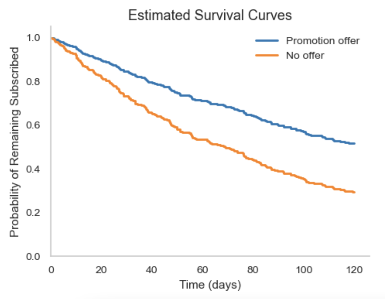
However, because this is a standard Cox model, the survival curves reflect associational rather than causal differences, meaning other factors not included in the model could explain part of the observed effect. Conditional survival curves such as this give the average survival probability over time for individuals with a specific covariate profile. They don’t give counterfactual survival. For example, what survival would have been had everyone received treatment $A$ versus treatment $B$. Estimating such causal survival curves requires specialized causal inference methods that simulate or estimate potential outcomes under different treatment strategies.
Causal Methods
Pooled Logistic Regression
Pooled logistic regression models discrete-time hazards using standard logistic regression. The key idea is to convert survival analysis into a classification problem. Rather than modeling the exact timing of an event, we break time into discrete intervals (e.g. days or weeks) and ask: Did the event happen in this interval, given that it hasn’t happened yet?. This involves restructuring the data so that each individual contributes one row per time period they were at risk, then fitting a standard logistic regression model (including time, treatment, and covariates). The model estimates the conditional probability of the event occurring at each interval, which serves as a discrete-time approximation of the hazard function:
\[\text{logit} \left[ P(Y_{it} = 1 \mid Y_{i,t-1} = 0, A_{i,t}, L_{i,t}) \right] = \beta_0(t) + \beta_A A_{i,t} + \beta_L L_{i,t}\]- $Y_{it}$: Indicator for event in interval t
- $A_{i,t}$: Treatment at t
- $L_{i,t}$: Covariates at t
- $\beta_0(t)$: Baseline hazard, modeled using time indicators or splines
By setting treatment to a fixed value across all individuals and time points, and predicting the hazards for each interval, you can construct counterfactual survival curves. This allows for direct estimation of causal effects, assuming time-varying confounding is appropriately controlled via covariate adjustment or inverse probability weighting.
Steps:
-
Reshape data Structure the dataset so each person contributes one row per time period they are at risk, stopping at the time of the event or censoring.
-
Fit pooled logistic regression Estimate the probability of the event occurring in each interval using logistic regression with time indicators, treatment, and time-varying covariates.
-
Simulate counterfactual survival To estimate survival under a fixed treatment strategy, set treatment to the desired level for all rows and compute predicted hazards:
\[\hat{S}(t) = \prod_{k=1}^t (1 - \hat{h}(k))\]where $\hat{h}(k)$ is the predicted hazard (probability of the event) at time k. Simulating under different treatment strategies yields causal survival curves.
Example
Suppose we want to estimate the effect of sending weekly promotional emails on time to unsubscribe. We have data on 500 users tracked weekly for up to 12 weeks. Each week, we observe:
- Whether a user received a promotion ($A_t$)
- Their engagement status ($L_t$)
- Whether they unsubscribed ($Y_t$)
First we need to reshape the data (convert to long format, so each row is one user-week observation, stopping at unsubscribe or censoring). Then we can model the discrete-time hazard (probability of unsubscribe) as a function of: week indicators (to flexibly model baseline hazard over time); treatment at that week; and engagement status at that week. For example, it might look something like: glm(Y ~ factor(week) + A + L, family = binomial, data = long_data).
Simulating Counterfactual Survival Curves
Now we can estimate survival under fixed treatment strategies (always send promos vs never send promos):
-
Create counterfactual datasets: Copy the original long dataset twice:
- In one copy, set $A_t = 1$ for all user-weeks (always send promotions)
- In the other, set $A_t = 0$ for all user-weeks (never send promotions)
Keep $L_t$ and time variables as observed or appropriately updated depending on assumptions (e.g., time-varying covariates can be set to observed or fixed values depending on the method).
-
Predict hazards: Use the fitted model to predict the probability of unsubscribing each week for every user in each counterfactual dataset:
\[\hat{h}_{i,t} = P(Y_{i,t} = 1 \mid Y_{i,t-1} = 0, A_{i,t}, L_{i,t})\] -
Calculate survival probabilities: For each user, calculate the survival probability at each week $t$:
\[\hat{S}_{i}(t) = \prod_{k=1}^t (1 - \hat{h}_{i,k})\] -
Aggregate over users: Average these individual survival probabilities across all users to get the estimated survival curve under each treatment strategy:
\[\hat{S}(t) = \frac{1}{N} \sum_{i=1}^N \hat{S}_i(t)\]
Plotting survival_always and survival_never over weeks shows the estimated probability of remaining subscribed under each promotional strategy. The difference between curves reflects the causal effect of sending weekly promotional emails on retention, assuming no unmeasured confounding and correct model specification. Keep in mind, the causal conclusions still depend on assumptions like no unmeasured confounding and correct model specification.
Inverse Probability of Censoring Weighting (IPCW)
IPCW adjusts for informative censoring by reweighting observed individuals based on the inverse of their probability of remaining uncensored.
Steps:
- Fit a model for censoring probability at each time $t$, conditioning on covariate and treatment history.
- Compute stabilized weights:
- Apply these weights in the outcome model (e.g. pooled logistic or Cox) to obtain unbiased estimates of treatment effects.
Marginal Structural Models (MSMs)
MSMs estimate causal effects of treatment strategies when treatment and confounders vary over time, and treatment affects future confounders.
Use inverse probability of treatment and censoring weights to adjust for time-varying confounding:
\[w_{i} = \prod_{k=1}^t \frac{P(A_{i,k} \mid A_{i,1:k-1})}{P(A_{i,k} \mid A_{i,1:k-1}, L_{i,1:k})} \times \frac{P(C_{i,k} = 0)}{P(C_{i,k} = 0 \mid A_{i,1:k-1}, L_{i,1:k-1})}\]Then, fit a weighted outcome model such as:
\[\text{logit} \left[ P(Y_{it} = 1 \mid A_{i,t}) \right] = \beta_0(t) + \beta_A A_{i,t}\]Parametric g-Formula
The parametric g-formula estimates causal effects by explicitly modeling the full joint distribution of the data and simulating counterfactual outcomes under different treatment strategies.
Steps:
-
Fit models for:
- Covariates $L_t$
- Treatment $A_t$
- Event $D_t$
- Censoring $C_t$
-
Simulate full individual trajectories under specified treatment regimes.
-
Compute survival probabilities under each regime and compare them to estimate causal effects.
Notes on Survival Models
Survival analysis methods must accommodate right censoring, which commonly arises due to fixed end-of-study follow-up. Some key distinctions:
- Nonparametric models (e.g., Kaplan-Meier) make no assumptions about the event time distribution.
- Parametric models (e.g., exponential, Weibull) assume a specific distribution.
- Semi-parametric models (e.g., Cox) do not assume a specific distribution for the baseline hazard but do impose structure on how covariates affect it.
Pooled logistic regression is a parametric model for discrete time, whereas Cox models are semi-parametric.
Comparison of methods
| Method | Purpose | Adjusts for | Handles Time-varying | Supports Causal Inference |
|---|---|---|---|---|
| Kaplan-Meier | Compare survival curves | No | No | No |
| Cox model | Estimate hazard ratios | Some | With extensions | Only under strong assumptions |
| Pooled Logistic | Flexible discrete hazard model | Yes | Yes | Yes (with g-formula or MSM) |
| IPCW | Adjust for censoring bias | Yes | Yes | Yes |
| MSM | Estimate marginal causal effects | Yes | Yes | Yes |
| Parametric g-Formula | Simulate counterfactual outcomes | Yes | Yes | Yes |
Preparing Data for Time-to-Event Analysis
Survival-style models require:
- A defined start time (e.g. treatment date, onboarding).
- A follow-up period and a time-to-event or censoring indicator.
- Proper handling of time-varying covariates.
The data is typically transformed to either:
- Wide format: with a single row per subject and time-to-event.
- Long format (person-period): where each individual contributes one row per time interval (day/week/month), allowing time-varying covariates or exposures.
Confidence Intervals for Causal Time-to-Event Models
Causal estimates from time-to-event models require valid uncertainty estimates. Common methods:
-
Robust (sandwich) standard errors: When using discrete-time models like pooled logistic regression, your dataset includes multiple rows per subject (one per time interval). Standard errors from basic regression assume independence across rows, which is violated in this structure. Robust (sandwich) variance estimators adjust for within-subject correlation, producing valid standard errors even when residuals are not independent. They’re easy to implement using cluster-robust standard errors or generalized estimating equations (GEEs), depending on the software.
-
Bootstrap methods: Bootstrapping involves resampling entire individuals (not rows) with replacement, refitting the model for each sample, and computing the variability of the causal estimand across replicates (creating an empirical distribution for confidence intervals). This automatically incorporates uncertainty due to model fitting, censoring, and time-varying treatment or covariates. This is particularly important when using IPW, IPCW, or MSMs, since packages may not account for the uncertainty in estimated weights. Bootstrap methods are more computationally intensive but are generally more robust for complex estimands, such as risk differences or simulated counterfactual survival curves.
-
Delta method: Used to approximate the standard error when transforming non-linear model parameters (e.g. log-hazard ratios to survival probabilities). It uses a first-order Taylor approximation to linearize the transformation and propagate uncertainty from the parameter estimates to the final quantity of interest. The delta method is especially useful when you want analytical confidence intervals without needing bootstrapping. However, it relies on asymptotic normality and may underestimate variance in small samples or highly nonlinear settings.
Even with valid standard errors, misspecified models (e.g. incorrect functional forms for time, non-proportional hazards, omitted confounders), can lead to biased point estimates and misleading confidence intervals. Confidence intervals only reflect precision, not accuracy. It’s critical to assess model assumptions and conduct sensitivity analyses where possible.
Effect heterogeneity over time
The causal effect of a treatment or exposure may not be constant throughout the entire follow-up period. Instead, the treatment effect can vary at different time points, meaning there is effect heterogeneity over time (time-varying treatment effects). Accounting for this heterogeneity is crucial for understanding when and how an intervention exerts its influence, which can inform better decisions.
Several approaches allow estimation of time-varying treatment effects:
- Interaction terms with time: In models like Cox or pooled logistic regression, including interaction terms between treatment and functions of time (e.g., time indicators, splines) permits the effect to change flexibly over follow-up.
- Stratified analyses: Estimating treatment effects separately in predefined time intervals can reveal how effects evolve.
- Flexible machine learning methods: Techniques such as time-varying coefficient models, dynamic survival models, or causal forests can capture complex heterogeneity patterns without strong parametric assumptions.
Effect heterogeneity over time can be visualized by plotting estimated hazard ratios, survival differences, or cumulative incidence differences across time points. These dynamic estimates help identify critical periods when treatment is most or least effective, supporting targeted intervention strategies or monitoring plans.
Other common methods
Mediation analysis
Mediation analysis is a statistical technique used to understand the mechanism or causal pathway by which a treatment (or exposure) influences an outcome through an intermediate variable known as the mediator. Rather than simply estimating whether a treatment affects an outcome, mediation analysis seeks to quantify \(\text{how much}\) of this effect occurs \(\text{directly}\) and \(\text{how much}\) is transmitted \(\text{indirectly}\) through the mediator.
Key concepts
- Treatment (or exposure), \(T\): The variable or intervention whose effect on the outcome we want to study.
- Mediator, \(M\): An intermediate variable that lies on the causal path between treatment and outcome.
- Outcome, \(Y\): The final variable of interest that we want to explain or predict.
Goals
The primary goal of mediation analysis is to decompose the total effect of the treatment on the outcome into two components:
- Direct effect: The portion of the treatment effect on the outcome that is not transmitted through the mediator. This captures pathways where treatment influences the outcome independently of the mediator.
- Indirect effect: The portion of the treatment effect that operates through the mediator. This represents the causal pathway where treatment changes the mediator, which in turn affects the outcome.
Mathematically, this decomposition helps to clarify how the treatment brings about change in the outcome, offering richer insights beyond the average treatment effect (ATE).
Typical workflow
Mediation analysis is generally conducted on individual-level data collected in a single study or experiment. The most common approach involves a series of regression models to estimate direct and indirect effects:
-
Estimate the total effect of \(T\) on \(Y\):
Fit a regression model predicting \(Y\) from \(T\) (and relevant covariates). The coefficient of \(T\) here captures the total effect. -
Estimate the effect of \(T\) on the mediator \(M\):
Fit a regression model predicting \(M\) from \(T\) (and covariates). This captures how the treatment influences the mediator. -
Estimate the effect of the mediator \(M\) on the outcome \(Y\), controlling for \(T\):
Fit a regression model predicting \(Y\) from both \(T\) and \(M\) (and covariates). The coefficient on \(M\) here captures the mediator’s effect on the outcome, while the coefficient on \(T\) estimates the direct effect. -
Calculate the indirect effect:
Multiply the effect of \(T \to M\) by the effect of \(M \to Y | T\) to estimate the indirect effect. Note, this approach only works if there’s no interaction between the mediator and treatment (i.e. the effect of the mediator on the outcome doesn’t vary by treatment level). See the next section for how to handle interactions. -
Calculate the direct effect:
The coefficient of \(T\) in the outcome model controlling for \(M\) is the direct effect. -
Inference and uncertainty:
Since the indirect effect is a product of two coefficients, its sampling distribution is usually non-normal. Bootstrapping or other resampling techniques are commonly used to estimate confidence intervals and test significance.
Other methods
Structural Equation Modeling (SEM)
A flexible framework that models direct and indirect pathways simultaneously using a system of structural equations, allowing for complex mediators and latent variables.
Causal Mediation Analysis
Uses counterfactual definitions of natural direct and indirect effects (e.g. the effect of treatment if the mediator were held fixed at its untreated value). These approaches allow for treatment-mediator interactions and enable more rigorous causal interpretation, under strong assumptions about ignorability.
Assumptions
For mediation analysis to yield valid causal interpretations, several assumptions must hold:
- No unmeasured confounding between treatment and outcome, treatment and mediator, and mediator and outcome (conditional on treatment and covariates).
- Correct model specification of the relationships between variables.
- No interference between units (treatment or mediator for one individual does not affect another).
- Temporal ordering: The mediator occurs after the treatment and before the outcome.
By carefully applying mediation analysis, researchers can gain insights not only about whether a treatment works, but also how it works, illuminating the causal mechanisms underlying observed effects.
Allowing interactions
When the effect of the mediator on the outcome varies by treatment level (i.e., there is a treatment-mediator interaction), standard linear decomposition (e.g. multiplying coefficients) may not give valid direct and indirect effects. In such cases, counterfactual-based methods (e.g., causal mediation analysis using potential outcomes) are more appropriate, as they allow for and estimate these interactions explicitly.
Meta mediation analysis
Meta-mediation extends this idea to a higher level. Instead of analyzing individual-level data, meta-mediation uses summary effect estimates from multiple independent experiments or studies (meta-experiments). It estimates how much of the variation in treatment effects on the outcome across experiments can be explained by variation in treatment effects on a mediator. In other words, meta-mediation performs mediation analysis across experiments, using the estimated treatment effects on the mediator and outcome from each experiment to infer causal mediation pathways at the meta-experiment level.
Suppose you have multiple experiments (meta-experiments), each perturbing some feature and measuring:
- An offline metric \(M\) (e.g., search relevance score),
- An online metric \(O\) (e.g., click-through rate),
- A final business KPI \(Y\) (e.g., revenue).
Our goal is to understand how much the offline metric \(M\) affects the business KPI \(Y\), and how much of this effect is mediated through the online metric \(O\).
Imagine \(n\) independent experiments, each producing estimated treatment effects on \(M\), \(O\), and \(Y\):
- \(\hat{\delta}_M^{(i)}\) = treatment effect on offline metric,
- \(\hat{\delta}_O^{(i)}\) = treatment effect on online metric,
- \(\hat{\delta}_Y^{(i)}\) = treatment effect on business KPI,
where \(i = 1, 2, \ldots, n\).
We assume the causal relations:
\[\hat{\delta}_O^{(i)} = \beta_{MO} \hat{\delta}_M^{(i)} + \epsilon_O^{(i)}\] \[\hat{\delta}_Y^{(i)} = \beta_{OY} \hat{\delta}_O^{(i)} + \epsilon_Y^{(i)}\]Here,
- \(\beta_{MO}\) is the causal effect of the offline metric on the online metric,
- \(\beta_{OY}\) is the effect of the online metric on the business KPI,
- \(\epsilon_O^{(i)}\), \(\epsilon_Y^{(i)}\) are noise terms.
Two-Stage Regression
We perform two regressions across the meta-experiments:
- Regress \(\hat{\delta}_O\) on \(\hat{\delta}_M\):
- Regress \(\hat{\delta}_Y\) on \(\hat{\delta}_O\):
The total mediated effect of the offline metric on the business KPI is estimated by the product:
\[\hat{\beta}_{\text{total}} = \hat{\beta}_{MO} \times \hat{\beta}_{OY}\]Estimating Confidence Intervals (CIs) Using Bootstrap
Because the total effect is a product of two regression coefficients, its uncertainty is non-trivial. To estimate CIs:
- Resample the meta-experiments with replacement many times (e.g., 1000 bootstraps).
- For each bootstrap sample:
- Recompute \(\hat{\beta}_{MO}\) and \(\hat{\beta}_{OY}\),
- Compute the product \(\hat{\beta}_{MO} \times \hat{\beta}_{OY}\).
- Use the empirical distribution of these products to derive confidence intervals, typically by taking the 2.5th and 97.5th percentiles for a 95% CI:
Interpretation
- \(\hat{\beta}_{MO}\) quantifies how changes in the offline metric affect the online metric.
- \(\hat{\beta}_{OY}\) quantifies how changes in the online metric affect the business KPI.
- Their product \(\hat{\beta}_{\text{total}}\) captures how the offline metric ultimately influences the business KPI through the online metric.
- Bootstrapped confidence intervals reflect uncertainty from both regression steps and their interaction.
Assumptions
This meta-mediation approach relies on several key assumptions to produce valid causal estimates:
-
Randomization and No Unmeasured Confounding
Each experiment in the meta-analysis is assumed to be a randomized controlled trial or equivalent, ensuring that treatment assignment is independent of potential outcomes. This justifies interpreting estimated effects \(\hat{\delta}_M^{(i)}, \hat{\delta}_O^{(i)}, \hat{\delta}_Y^{(i)}\) as unbiased causal effects. -
Linearity and Additivity of Effects
\[\hat{\delta}_O^{(i)} = \beta_{MO} \hat{\delta}_M^{(i)} + \epsilon_O^{(i)}\] \[\hat{\delta}_Y^{(i)} = \beta_{OY} \hat{\delta}_O^{(i)} + \epsilon_Y^{(i)}\]
The model assumes a linear relationship between the offline metric and the online metric, and between the online metric and the business KPI:This means the mediation is additive and effects do not vary nonlinearly or interact with other unmodeled factors.
-
No Direct Effect of Offline Metric on Business KPI Outside the Mediator
The framework assumes that all causal influence of the offline metric \(M\) on the business KPI \(Y\) operates through the online metric \(O\) (the mediator). There is no unmodeled direct pathway from \(M\) to \(Y\) that bypasses \(O\). -
Independent and Identically Distributed (i.i.d.) Errors
The noise terms \(\epsilon_O^{(i)}\) and \(\epsilon_Y^{(i)}\) are assumed to be independent across experiments and have mean zero. This justifies the use of standard regression techniques and bootstrap inference. -
Sufficient Variation Across Experiments
The meta-experiments must provide enough variation in the treatment effects on \(M\) and \(O\) to reliably estimate the regression coefficients \(\beta_{MO}\) and \(\beta_{OY}\). -
Stable Unit Treatment Value Assumption (SUTVA)
There are no interference effects between units or experiments — that is, the treatment effect for one experiment is unaffected by others.
Violations of these assumptions can bias estimates or invalidate confidence intervals. For example, if the offline metric affects the business KPI through pathways other than the online metric, the mediation estimate will be incomplete. Similarly, unmeasured confounding or nonlinear effects require more advanced methods beyond this linear meta-mediation framework.
Summary
Meta-mediation can estimate how a treatment’s effect on an upstream (offline) metric transmits through a mediator (online metric) to impact a final outcome (business KPI). It focuses on decomposing causal pathways using aggregated effects from multiple experiments.
This methodology helps organizations understand which offline improvements lead to better business outcomes by driving changes in online metrics, guiding metric prioritization and investment. In practice, you often use propensity scores or matching to reduce confounding before performing mediation analysis, or you use IV methods to address confounding in mediator or treatment assignment when needed.
Surrogate/Proxy Validation
In randomised experiments, we often rely on short-term proxy or surrogate metrics as stand-ins for more important but harder to measure outcomes (e.g. north stars like long term retention or revenue). Validating whether a proxy reliably predicts the true outcome across multiple experiments is critical for trustworthy decision-making. However, a common challenge is measurement error: each experiment’s estimated treatment effect on the proxy metric is noisy, and this noise can be correlated with the noise in the estimated effect on the north star metric (in the same experiment). This correlation can bias naïve regressions relating proxy effects to outcome effects, typically attenuating estimates (biasing towards zero), and obscuring true relationships.
To correct for this bias, the leave-one-out instrumental variable (LOO-IV) method leverages the logic of instrumental variables but in a meta-analytic context. Instead of estimating treatment effects, it focuses on the relationship between proxy and outcome effect estimates across experiments. The key idea is to construct an instrument by removing the noisy estimate from the experiment in question, thus creating a proxy measure that is correlated with the true effect but uncorrelated with the noise in that experiment’s outcome estimate.
Steps
-
Collect summary statistics from multiple experiments: For each experiment $i$, obtain:
- $\hat{\beta}_{\text{proxy}, i}$: Estimated treatment effect on the proxy metric.
- $\hat{\beta}_{\text{outcome}, i}$: Estimated treatment effect on the outcome (north star) metric.
-
Construct the leave-one-out instrument: For each experiment $i$, compute:
\[Z_i = \frac{1}{N - 1} \sum_{\substack{j=1 \\ j \neq i}}^{N} \hat{\beta}_{\text{proxy}, j}\]This is the average proxy effect excluding experiment $i$.
-
First-stage regression (predict proxy effect): Regress the noisy proxy effect on the instrument:
\[\hat{\beta}_{\text{proxy}, i} = \pi_0 + \pi_1 Z_i + u_i\] -
Second-stage regression (predict outcome effect): Use predicted proxy effects from step 3 to regress on outcome effects:
\[\hat{\beta}_{\text{outcome}, i} = \alpha + \gamma \hat{\beta}_{\text{proxy}, i}^{\text{pred}} + \varepsilon_i\] -
Interpretation: The coefficient $\gamma$ estimates how changes in the proxy metric relate to changes in the true outcome metric, corrected for measurement error in the proxy.
Example
Imagine you run 50 A/B experiments testing UI changes. Each experiment reports:
- The estimated impact on click-through rate (CTR): the proxy metric.
- The estimated impact on long-term retention: the north star metric.
Because CTR estimates are noisy and measured on the same users as retention, simply regressing retention effects on CTR effects underestimates the true relationship. Using the leave-one-out method, for each experiment:
- Compute the average CTR effect from the other 49 experiments.
- Use this as an instrument to isolate the “true” CTR effect.
- Then regress retention effects on the predicted CTR effects from the first stage.
This approach produces an unbiased estimate of how well CTR predicts retention changes, helping decide if CTR is a valid proxy for long-term success.
Summary
The leave-one-out instrumental variable method provides a practical and flexible way to validate surrogate or proxy metrics across multiple experiments by correcting for correlated measurement error. It does not require the strong homogeneity assumptions of other methods and is especially useful when experiments are heterogeneous and noise levels vary.
Conclusion
Causal inference is inherently difficult because its core assumptions are untestable. Unlike predictive modeling, where performance can be evaluated against ground truth, causal analyses always carry the risk of bias, whether from unmeasured confounding, model misspecification, or violated identification assumptions. You’ll always get a result, and it may look reasonable, but that doesn’t mean it’s correct. That’s why interpretation, sensitivity analysis, and clear communication about what the result does and does not mean are essential.
In industry, where the pressure to move fast is intense, this kind of careful consideration often gets overlooked. Even if it’s just a quick whiteboard exercise, sketching a causal graph early on can be invaluable. Bring in both product and technical stakeholders to help surface and challenge assumptions, and keep a copy to refer back to. Adding notes on the expected direction of effects (i.e. a signed graph) can also help avoid hindsight bias or post-hoc rationalizations.
A common pushback to this structured approach is: “Shouldn’t we let the data speak for itself instead of assuming?” While tempting, the data alone usually can’t answer causal questions. Observing an association between A and B doesn’t reveal whether A causes B, B causes A, or if both are driven by some unmeasured third factor. In most cases, domain knowledge is essential to build a plausible causal structure. That said, some situations, such as natural experiments, time ordering, or policy changes, can provide useful leverage.
It can be discouraging to realize how rarely we can identify effects with full confidence from observational data. However, even imperfect causal estimates can be valuable. When decisions must be made under uncertainty, thoughtful causal reasoning is far better than ignoring causality altogether.
Appendix
Commonly Confused Terms
| Term | Meaning in One Field | Common Confusion or Contrast |
|---|---|---|
| Marginal effect | In epidemiology/econometrics: average population-level effect | In ML/stats: partial derivative in a GLM or change in outcome for one unit change in input |
| Conditional effect | In ML: subgroup-specific (e.g. CATE) | Often confused with marginal effects; reverse meanings in some contexts |
| Confounder | In causal inference: common cause of treatment and outcome | In industry: sometimes any variable correlated with outcome |
| Collider | Variable caused by both treatment and outcome | Often mistaken for a confounder — adjusting for it introduces bias |
| Interaction | In regression/ML: product term between variables | In causal inference: may imply effect heterogeneity (CATE) |
| Effect modification / Moderation | Heterogeneity of effect by subgroup | Often confused with mediation (i.e., how vs. for whom an effect occurs) |
| Mediation | Effect through an intermediate variable | Mistaken for moderation (effect heterogeneity); needs different methods |
| Instrument / IV | Valid instrument must satisfy exclusion + relevance assumptions | In industry, often misapplied to any “natural variation” |
| Propensity score | Treatment probability used for balancing | Sometimes misused as a predictor or feature in a non-causal model |
| Exchangeability | Assumption that potential outcomes are independent of treatment given covariates | Often confused with covariate balance or random sampling |
| Selection bias | Bias from conditioning on a collider or restricted sample | In industry, used loosely to mean any sample skew |
| Surrogate / Proxy | Stand-in for a hard-to-measure outcome | Risk of invalid inference if it’s not a valid surrogate |
| Model | In ML: a predictive system (e.g., neural net) | In causal inference: often an estimation tool based on assumptions |
| Bias | In ML: systematic prediction error | In causal inference: failure to estimate the true causal effect due to confounding or misspecification |
do-calculus
Up to now, I’ve focused on the potential outcomes framework. The do-calculus framework offers a complementary graph-based approach to causal inference, providing formal rules to determine when and how causal effects can be identified from observational data using a causal DAG. The rules rely on altering the graph by “cutting” edges to represent interventions (removing incoming arrows to nodes intervened upon) or blocking paths.
- The notation \(do(X = x)\) represents an intervention that sets the variable \(X\) to value \(x\), rather than simply observing \(X = x\). This aligns with the potential outcomes idea of comparing outcomes under different treatments.
- The goal is to estimate the causal effect: \(P(Y \mid do(X = x))\), which is the distribution of outcomes we would expect if we were to intervene and set \(X = x\). In observational data, this is not generally equal to \(P(Y \mid X = x)\) due to confounding or selection bias.
- Do-calculus uses the structure of a causal DAG to determine whether and how we can express \(P(Y \mid do(X = x))\) in terms of observed data distributions.
- There are 3 general rules that allow us to systematically convert interventional queries into expressions that can be computed from observational data (when such identification is possible). In practice, you often apply the three rules multiple times in sequence to simplify complicated interventional distributions into expressions involving only observed data.
| Rule | Name | Purpose | Graphical Condition | PO Analogy | Effect on Expression |
|---|---|---|---|---|---|
| Rule 1 | Insertion/deletion of observations | Drop or add observed variable from conditioning set | \(Y \perp Z \mid X, W \text{ in } G_{\text{do}(X)}\) | Ignoring irrelevant covariates | \(P(Y \mid do(X), Z, W) = P(Y \mid do(X), W)\) |
| Rule 2 | Action/observation exchange | Replace \(do(Z)\) with conditioning on \(Z\) | \(Y \perp Z \mid X, W \text{ in } G_{\text{do}(X), \overline{Z}}\) | Treating observed covariates as fixed treatments | \(P(Y \mid do(X), do(Z), W) = P(Y \mid do(X), Z, W)\) |
| Rule 3 | Insertion/deletion of actions | Remove unnecessary intervention | \(Y \perp Z \mid X, W \text{ in } G_{\text{do}(X), \overline{Z(W)}}\) | Dropping irrelevant treatment terms | \(P(Y \mid do(X), do(Z), W) = P(Y \mid do(X), W)\) |
Here, \(G_{\text{do}(X)}\) denotes the causal graph after intervening on \(X\) (removing incoming edges into \(X\)), and \(G_{\text{do}(X), \overline{Z}}\) denotes the graph after intervening on \(X\) and removing outgoing edges from \(Z\).
The backdoor and frontdoor criteria are specific applications of do-calculus that give usable adjustment formulas without needing to chain all 3 rules manually:
1. Backdoor Criterion
If there exists a set of variables \(Z\) that blocks all backdoor paths from \(X\) to \(Y\) (paths that end with an arrow into \(X\)), and no member of \(Z\) is a descendant of \(X\), then:
\[P(Y \mid do(X = x)) = \sum_z P(Y \mid X = x, Z = z) P(Z = z)\]This corresponds to covariate adjustment in the potential outcomes framework (exchangeability conditional on \(Z\)).
2. Frontdoor Criterion
When no set of confounders exists that can block backdoor paths from \(X\) to \(Y\) (e.g., due to unmeasured confounding), but there is a mediator \(M\) that fully transmits the effect of \(X\) on \(Y\), and there are no unmeasured confounders affecting both \(X\) and \(M\) or \(M\) and \(Y\), the frontdoor adjustment formula applies:
\[P(Y \mid do(X = x)) = \sum_m P(M = m \mid X = x) \sum_{x'} P(Y \mid M = m, X = x') P(X = x')\]This works by first estimating the causal effect of \(X\) on \(M\), then the effect of \(M\) on \(Y\) while holding \(X\) constant, and combining these to recover the unbiased effect of \(X\) on \(Y\). The validity of this approach depends on the absence of confounding between \(X\) and \(M\), and on \(X\) blocking all backdoor paths from \(M\) to \(Y\). Essentially, the frontdoor criterion applies the backdoor adjustment consecutively to these two causal steps. Given it has very strong assumptions and requires a specific causal structure, this is less commonly used in practice.
Assumptions
Do-calculus assumes a correct and complete causal DAG. Omitted variables or misspecified directions can lead to wrong conclusions. It cannot fix issues with measurement error, selection bias unrelated to the graph structure, or violations of consistency. Several packages (like DoWhy or CausalInference in Python) implement do-calculus identification algorithms to automate these calculations.
References / further reading
-
Hern´an MA, Robins JM (2020). Causal Inference: What If. Boca Raton: Chapman & Hall/CRC.
-
Malcolm Barrett, Lucy D’Agostino McGowan, Travis Gerke (2025). Causal Inference in R
-
Inoue, K., Goto, A., Sugiyama, T., Ramlau-Hansen, C. H., & Liew, Z. (2020). The Confounder-Mediator Dilemma: Should We Control for Obesity to Estimate the Effect of Perfluoroalkyl Substances on Health Outcomes? Toxics, 8(4), 125. https://doi.org/10.3390/toxics8040125