Population estimates: one sample standard errors and confidence intervals
Often we calculate point estimates for a population based on a sample of data (e.g. the mean). How confident should we be in those estimates? Well, one quantifiable source of error is the sampling error. This is the variation in the estimate caused by random selection. In this post I’ll explain how the central limit theorem and sampling distributions allow us to quantify the sampling error, and how to communicate the uncertainty of an estimate using a confidence interval.
Motivating example: how much does a kangaroo weigh?
Let’s say I work on a wildlife reserve and I want to know the average weight of adult kangaroos in my reserve. This is an expensive and difficult exercise, so I can’t weigh them all. Instead, I go out and randomly pick 10 adult kangaroos and weigh them. The average weight is 45.3kg. Now I go out again the next day and find the average is 46.9kg. If you think about it, this is expected. Every time we take a random sample, we expect some variation just by chance (the sampling error). It’s even possible that just by chance I get unlucky and pick the 10 heaviest (or the 10 lightest) kangaroos one day.
Sampling distribution
So what if I repeat that exercise many times? Intuitively, the estimates should vary around the true estimate, so the mean of that distribution will converge to the true mean value as the number of estimates increases (this is the law of large numbers). The distribution of estimates (means in this case) is what we call the sampling distribution of the estimator. Below I show what this looks like if we plot the mean estimates from 30 days (each time weighing 10 kangaroos), 100 days, and 1000 days. As the number of estimates increases, it looks more and more normal (bell curve). This is what the Central Limit Theorem (CLT) tells us: as n increases, the distribution converges to the normal distribution (with the same mean as the population, but a smaller variance).

This means that some days I’ll get a very low estimate, others a high estimate, but on average it’s around 46kg. The fact that it converges to a normal distribution centered on the mean is an extremely useful property. I’ll explain why next. First, note the CLT does come with some assumptions:
- the data is a random sample;
- each value is independent (they don’t influence each other);
- the sample size is not >10% if the sampling is without replacement; and,
- the sample size is sufficiently large.
Standardising
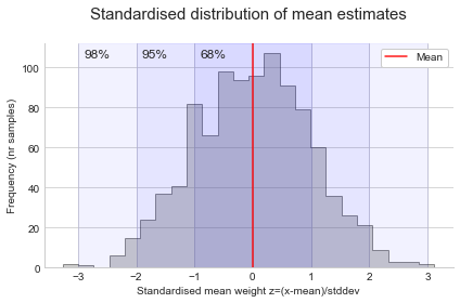
Standardising the sampling distribution allows us to talk more generally about the probability of different estimates. To create the standardised values, Z, we take the difference between each x value and the mean, and divide by the standard deviation:
\[Z = \frac{x - \mu}{\sigma}\]Z has a mean of 0 and standard deviation of 1, and is normally distributed (as X was normally distributed). Plotting the values of Z, we can easily see the 68-95-98 rule: 68% is within 1 standard deviation of the mean, 95% is within 2 standard deviation of the mean, and 99.7% is within 3 standard deviation of the mean.

Summarising the sampling distribution
There are two common ways to summarise the sampling distribution:
- 1) The standard error: a measure of the variability in the sampling distribution, or how far off we expect an estimate to be off on average. As n increases, the standard error decreases. Not to be confused with standard deviation (variability in a measured quantity). Note, the population standard deviation ($\sigma$) is not usually known, so it’s usually estimated with the sample standard deviation (s).
- 2) Confidence interval (CI): a range that includes a given fraction of the sampling distribution. E.g. the 95% CI is the range from the 2.5th to 97.5th percentiles (5% split on either side). When explaining to a non-technical audience, we’ll normally say something like we’re reasonably confident that the true value is somewhere within the CI range, or this is a range of plausible values for the true value. However, don’t misinterpret the confidence. We’re measuring how reliable our estimate is, based on how much estimates would vary across repeated experiments. So there isn’t a 95% probability the actual value falls within the confidence interval. Rather, 95% of the time (if we repeat our sampling process), we get a confidence interval that contains the true value. In the other 5% the true value is not in the CI at all (i.e. 1/20 experiments I’m wrong and return a CI that doesn’t contain the true value).
Where ‘s’ is the sample standard deviation, and the critical value ‘z’ is based on our selected confidence. E.g. z=1.96 for 95% confidence. The z value comes from looking at the standardised sampling distribution and calculating how many standard deviations do we need to have the area under the curve cover 95% of values. E.g. we saw earlier that for 65% we would only need +/-1 standard deviation, and for 95% we need ~2 (it’s actually 1.96 to be precise, which is the critical z above).
Confidence interval for the mean estimate
Now, coming back our example. In reality, we don’t want to repeat the sampling many times. We want to take that first estimate from one day of weighing 10 kangaroos (45.3kg), and understand how confident we should be that this is accurate. To do that we’ll create a confidence interval based on what we learned above:
import numpy as np
np.random.seed(26)

# Create a sample of 10 weights based on a normal distribution (mu=46, sigma=3)
single_day_measurements = np.random.normal(46, 3, 10)
sample_mean = np.mean(single_day_measurements)
sample_std_dev = np.std(single_day_measurements, ddof=1)
n = len(single_day_measurements)

se = sample_std_dev / np.sqrt(n)
moe = 1.96 * se
ci_lower, ci_upper = (sample_mean - moe), (sample_mean + moe)

print('Estimated mean = {:.2f}'.format(sample_mean))
print('Estimated standard deviation = {:.2f}'.format(sample_std_dev))
print('Standard error = {:.3f}'.format(se))
print('Margin of error = {:.3f}'.format(moe))
print('95% CI = ({:.2f}, {:.2f})'.format(ci_lower, ci_upper))

Estimated mean = 45.31
Estimated standard deviation = 2.91
Standard error = 0.921
Margin of error = 1.804
95% CI = (43.51, 47.12)
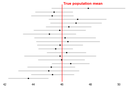
So based on this sample, we estimate the population mean is somewhere in the range 43.5 to 47.1kg with 95% confidence. To make sure the interpretation is clear, the plot below repeats this exercise 20 times and shows the resulting confidence intervals compared to the true population mean (not known in reality). Notice that 19 of the confidence intervals overlap with the mean, but 1 does not. This matches our expectation that 19/20 times (95%) our estimation process works and produces a confidence interval that contains the mean, but 1/20 times (5%) it does not.

Complete Python code and formulas: estimating a population mean
Note, if the population standard deviation isn’t known and the sample size is small (<30), we can use the t-distribution to determine the critical value instead of z. Like the normal distribution, the t-distribution is symmetric and bell shaped, but it has heavier tails (more values at the extremes, so values far from the mean more common than for z). However, for large n the t-distribution becomes very close to the z distribution, so it’s a safe bet in general to pick t instead of z. Below I’ll show how to use both methods in Python.
Mean: using z distribution
Note, the population standard deviation ($\sigma$) below can be estimated with the sample standard deviation (s) if n>30 (else use the t-distribution shown next):
\[SE_\text{mean} = \frac{\sigma}{\sqrt{n}}\] \[CI_\text{mean} = \bar{x} \pm z \frac{s}{\sqrt{n}}\]Using base/scipy: 2 ways
import numpy as np
import scipy.stats as st

np.random.seed(26)
sample = np.random.normal(46, 3, 10)
sample_mean = np.mean(sample)
sample_stddev = np.std(sample, ddof=1)
n = len(sample)
alpha = 0.05
critical_val = st.norm.ppf(1-alpha/2)

se = sample_stddev/(n**0.5)
ci_lower, ci_upper = sample_mean-(critical_val*se), sample_mean+(critical_val*se)

print('95% CI = ({:.2f}, {:.2f})'.format(ci_lower, ci_upper))

st_se = st.sem(sample)
st_ci_lower, st_ci_upper = st.norm.interval(alpha=1-alpha,
                                            loc=sample_mean,
                                            scale=st_se
                                            )

print('95% CI with scipy = ({:.2f}, {:.2f})'.format(st_ci_lower, st_ci_upper))

95% CI = (43.51, 47.12)
95% CI with scipy = (43.51, 47.12)
Mean: using t distribution
\[CI_\text{mean} = \bar{x} \pm t_c \frac{s}{\sqrt{n}}\]import numpy as np
import scipy.stats as st
np.random.seed(26)
sample = np.random.normal(46, 3, 10)
sample_mean = np.mean(sample)
sample_stddev = np.std(sample, ddof=1)
n = len(sample)
alpha = 0.05
conf = 1 - (alpha / 2)
critical_val = st.t.ppf(conf, (n-1))
se = sample_stddev/(n**0.5)
ci_lower, ci_upper = sample_mean-(critical_val*se), sample_mean+(critical_val*se)
print('95% CI = ({:.2f}, {:.2f})'.format(ci_lower, ci_upper))
st_se = st.sem(sample)
st_ci_lower, st_ci_upper = st.t.interval(alpha=1-alpha,
loc=sample_mean,
scale=st_se,
df=n-1
)
print('95% CI with scipy = ({:.2f}, {:.2f})'.format(st_ci_lower, st_ci_upper))
95% CI = (43.23, 47.40)
95% CI with scipy = (43.23, 47.40)
Estimating a population proportion
One of the other common statistics we want to estimate for a population is a proportion (e.g. conversion rate). If the sample is large enough (np and n(1-p) are greater than 5), we can estimate a population proportion using the normal approximation:
\[SE_\text{p} = \sqrt\frac{\hat{p}(1-\hat{p})}{n}\] \[CI_\text{p} = \hat{p} \pm z*SE_\text{p}\]import numpy as np
import scipy.stats as st
from statsmodels.stats.proportion import proportion_confint
sample = [1,0,1,1,0,0,0,0]
sample_p = np.mean(sample)
n = len(sample)
alpha = 0.05
conf = 1 - (alpha / 2)
critical_val = st.norm.ppf(conf)
se = np.sqrt(sample_p*(1-sample_p)/n)
ci_lower, ci_upper = sample_p - critical_val*se, sample_p + critical_val*se
print('95% CI (using z) = ({:.2f}, {:.2f})'.format(ci_lower, ci_upper))
nr_successes = np.sum(sample)
nr_trials = len(sample)
alpha = 0.05
sm_ci_lower, sm_ci_upper = proportion_confint(count=nr_successes,
nobs=nr_trials,
alpha=alpha)
print('95% CI using statsmodels = ({:.2f}, {:.2f})'.format(sm_ci_lower, sm_ci_upper))
95% CI = (0.04, 0.71)
95% CI using statsmodels = (0.04, 0.71)
Bootstrapping: a universal approach
In the above examples we assumed the population distribution is normal, though they would also work for many other distributions if the sample is relatively large (based on CLT). However, bootstrapping is an alternative approach that makes no assumptions about the distribution. Instead, we simulate multiple experiments by resampling multiple times from the original sample (randomly selecting the same n each time, with replacement). For each new sample we calculate the statistic we are estimating (e.g. the mean), and save it. The distribution of these estimates gives us an estimate of the sampling distribution, and it’s standard deviation is an estimate of the standard error. If the distribution is normal, we can simply use the percentiles to get a CI (e.g. 2.5th and 97.5th percentiles for a 95% CI):
\[\text{Percentile CI} = 100*(\frac{\alpha}{2}), 100*1-(\frac{\alpha}{2})\]However, if it’s non-normal, we might over/underestimate the CI with this method, so it’s better to use a bias-correcting method (e.g. BCa). Read more on this here.
The downside of this method is that it can be slow, particularly if your working with large samples. However, there are some tricks for optimising it. Given it’s simplicity, I would recommend using it for your exploratory analysis. If you run into speed issues and your not able to find adequate optimisations, then you can always switch to the analytic methods discussed earlier.
Python implementation
TBD
Other sources of error
Note that in this post we talked about the sampling error, which causes variation in estimates due to the nature of taking a random sample. However, this is not the only source of error in estimation. Two other common sources of error are:
- Measurement error: error due to incorrect data entry. E.g. if you ask people for their weight, they may round the value, use an old measurement, or lie.
- Sample bias: when the sample isn’t a good representation of the population (e.g. not random).
In the above post we’ve only corrected for sampling error, so these other sources still need to be considered and corrected before you do your estimation.