Linear regression: theory review
Linear regression is a model for predicting a continuous outcome (dependent variable), from a set of features (independent variable/s). For example, you could use it on past home sales data to predict the price of a new listing. The outcome would be the sale price, and the predictors could be things like the number of bedrooms, and size of the house. While the true relationships between these features and the outcome in the real world are likely complex, we can often get a reasonable approximation with a simple additive linear model. If you think of each row in the data set as an equation, we want to figure out what (linear) combination of the features we should take to get a value as close as possible to the actual sale prices. Given it’s simplicity, efficiency and interpretability, it’s one of the most commonly used models in practice. It’s used for both prediction (e.g. predicting home sale prices), and understanding relationships (e.g. what factors drive a higher sale price?). However, it can produce biased estimates and inaccurate statistical inference when the assumptions are not met, so it’s important to properly review the model fit and interpret the results correctly. A warning, this is a very long post, mostly intended to be a reference for me when I want to refresh my memory.
Intuition
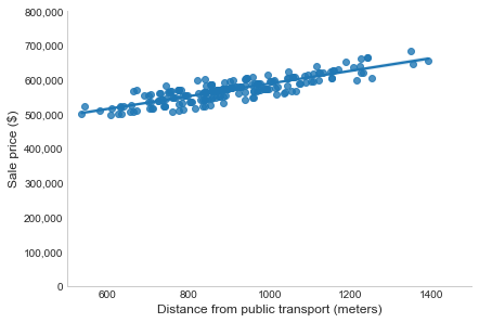
Imagine we have just one feature, the distance between the house and the nearest public transport. As demonstrated below, there is a linear relationship between this and the outcome: as the distance increases, so does the sale price (they have a positive correlation). Note, this doesn’t prove there is a causal relationship, as the correlation could be partially (or even fully) explained by other factors not accounted for (e.g. whether there’s a school nearby, or distance from the CBD). To predict the sale price of a house, we fit a line through these points, choosing the placement that minimises the distance between the actual prices and the predicted values (i.e. the vertical distance from each point to the line, called the residual). The line now gives us a predicted sale price for every distance from public transport. For a new listing we would look up the distance from public transport and just take the corresponding price from the line.
When we have multiple features, we’re doing the same thing but in a multi-dimensional space. Instead of a line, we fit a hyperplane. This is why we use the term “linear”, as we’re only using lines and planes (i.e. linear functions of the inputs). There are a number of ways to measure the closeness of the actual and predicted values (residuals), but the most common is the least squares criterion used in Ordinary Least Squares (OLS).
Ordinary Least Squares (OLS)
OLS finds the combination of the features that minimises the sum of the squared residuals (RSS). Let’s break that down. Given the feature values (X’s), we want to determine the weights (coefficients or \(\beta\)), that when applied to our training data gives us a predicted values (\(\hat{Y}\)) as close as possible to the actual sale prices (Y). This makes it a supervised parametric model, as it requires the actual outcomes for the training data (supervised), and assumes a linear relationship between the features and the outcome with a fixed set of parameters (the coefficients, making it parametric). Giving the following:
\[\hat{Y} = \hat{\beta_0} + \hat{\beta_1} * X_1 + ... + \hat{\beta_n} * X_n\] \[Y = \beta_0 + \beta_1 * X_1 + ... + \beta_n * X_n + \epsilon\] \[\epsilon_i = y_i - \hat{y_i}\] \[RSS = \epsilon_1^2 + ... + \epsilon_n^2\]Where:
- \(\beta_0\) is the intercept (value of Y when all X=0). Without this we would assume Y=0 when all X=0 and force the line to pass through the origin (Y=0, X=0). This might not make sense, but can also bias the \(\beta_n\) coefficients. Including \(\beta_0\) allows the line to shift up/down the Y axis to pass through the middle of the points, reducing the error.
- \(\beta_n\) are the weights for each feature \(X_n\) (change in Y for a 1 unit change in X)
- \(\epsilon\) is the remaining error or unexplained variability in Y (residuals, i.e. distance between \(\hat{Y}\) and Y).
- To find the unknown \(\beta\)s that reduce the overall error, OLS minimises the sum of the squared residuals (RSS). Squaring the errors avoids positive and negative errors cancelling out, and puts more emphasis on larger errors (2 becomes 4 or doubles, 10 becomes 100 which is tenfold). This also provides a smooth and continuous function that can be minimised with different optimisation methods. However, this is not robust to outliers. We’re taking the sum of the squared errors, so an outlier can have a large effect and bias the coefficient (pulling the line away from most points). Outliers will need to be understood and handled.
How it works
Ideal case
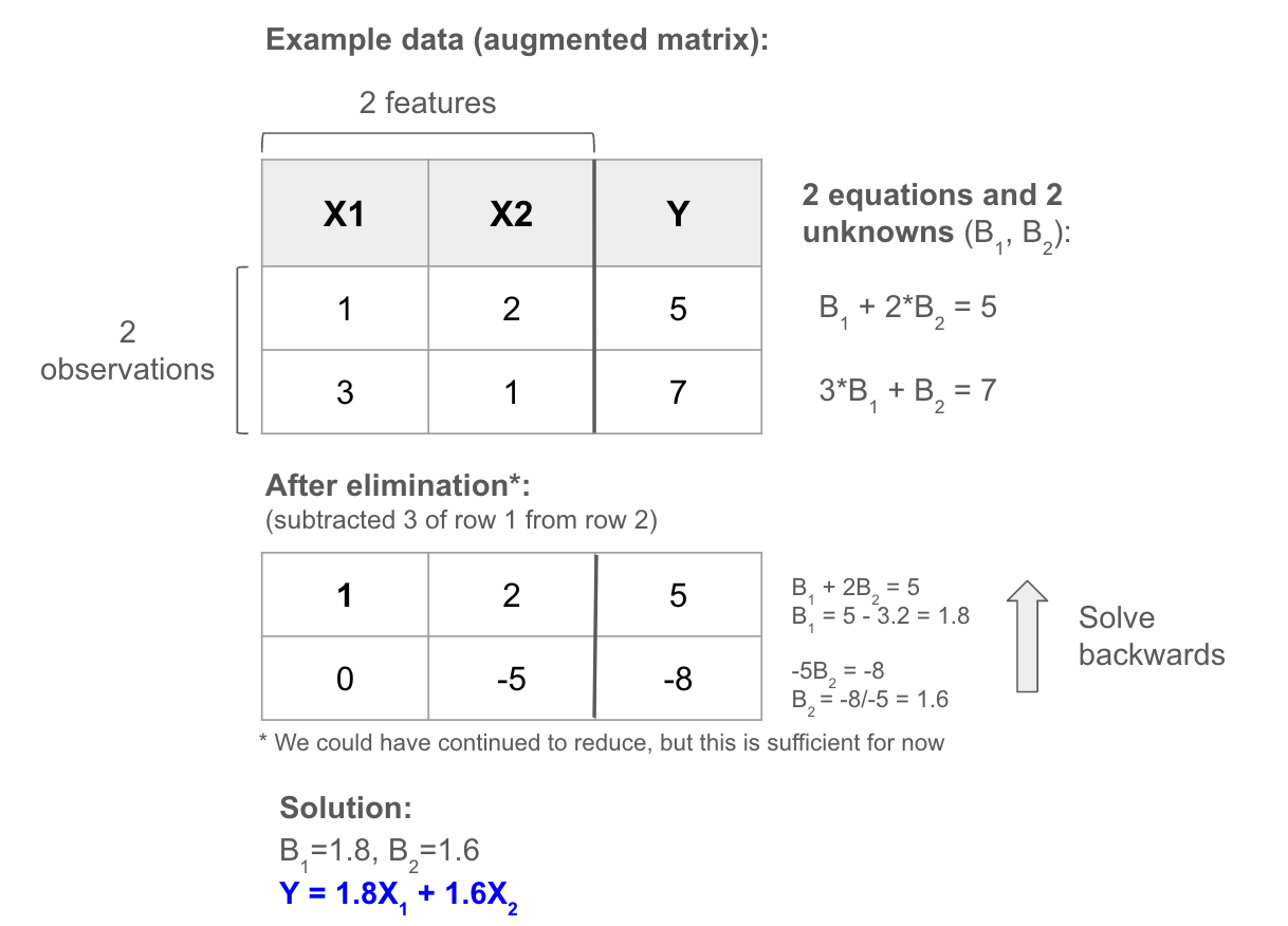
To understand how it works, let’s first create a play example where the outcome Y is a linear combination of the inputs X. The data set is just a matrix, so we can try to solve the system of linear equations with linear algebra using elimination. We simplify the equations by subtracting multiples of rows from each other (noting this doesn’t change the relationship between the X’s and Y as we’re doing the same to both sides), until we have an upper triangular matrix (0’s below diagonal). At that point, the last row has only one unknown, which we can easily solve knowing the output. Then we just work backwards up the triangle to solve the remaining, as each time there will be only one unknown (having solved the others).
To produce a single solution like this: Y must be a linear combination of the columns, and the rows and columns must be independent (i.e. we require a square invertible matrix). We more commonly have a tall thin matrix (more equations than unknowns), which will produce either 0 or 1 solution (any noise in the data would result in no solution). If the matrix is short and wide (more unknowns than equations), some columns are “free”, meaning they can take any value in the equations and so there will be infinite solutions.
Closest fit (reality)
Think of the geometric space filled by all linear combinations of the features (called the column space). If the outcome vector is in there (i.e. it’s a linear combination of the columns like above), we can find coefficients (feature weights) that will produce it with no error. However, it’s typically not (e.g. there’s some measurement error or missing factors), so we want to find the coefficients which give the ‘closest’ fit for our given output vector to minimize the error. Two common ways to do this for OLS are: the normal equation (closed form, one solution), and gradient descent (iterative algorithm).
Normal Equation
The normal equation is an explicit formula that directly computes the OLS estimates. We’ll use the linear algebra notation Ax=b, where A is the feature matrix, x is the vector of \(\beta\) coefficients, and b is the outcome vector (dependent variable). By projecting our outcomes b onto the column space (all linear combinations of the features), we find the part of b that can be explained by our features (let’s call this p, where p = a projection matrix * b), with some remaining error e (the gap between the outcomes and the projection, i.e. e=b-Ax). Mathematically we can prove that the error is minimised when it’s perpendicular (orthogonal) to the column space, which means A and e are perpendicular and equal 0 when multiplied. This fact allows us to solve for \(\hat{x}\) (the coefficients), giving the solution \(\hat{x}=(A^TA)^\text{-1} A^Tb\):
- The minimum error \(b-A\hat{x}\) is orthogonal to the column space \(A^T\), thus \(A^T(b-A\hat{x})=0\) which re-arranges to \(A^Tb = A^TA\hat{x}\). We multiply both sides by \((A^TA)^-1\) to eliminate \(A^TA\) (becomes the identity matrix) giving the solution \(\hat{x}=(A^TA)^\text{-1} A^Tb\).
- \(p=A\hat{x}=A(A^TA)^\text{-1}A^Tb=Pb\): p is the solveable part of b that’s in the column space (i.e. a linear combination of A that minimises the error). Thus \(A(A^TA)^\text{-1} A^T\) is the projection matrix P that projects b onto the column space of A.
- If all measurements were perfect, the error could be e=b-Ax=0, as there is an exact solution to Ax=b and the line goes straight through the points (in this case the projection Pb returns b itself as that is the closest).
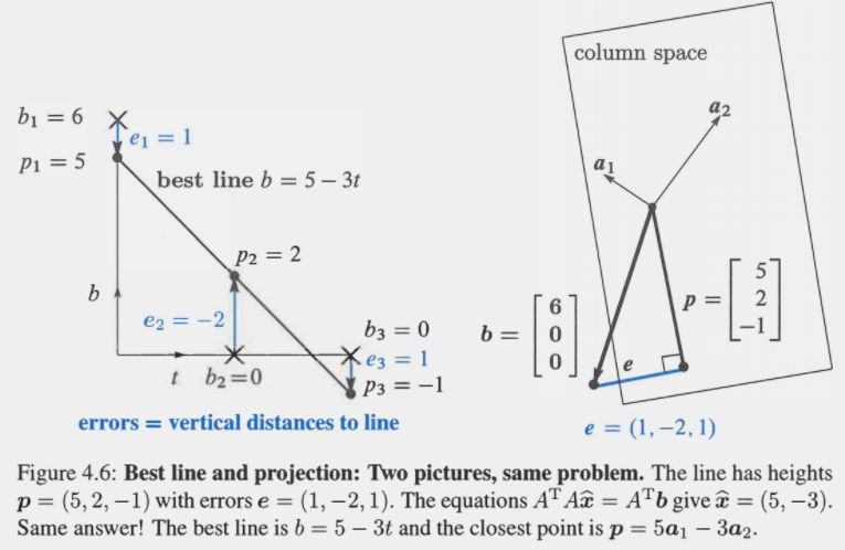
We can see how this works visually in the example below (left side shows fitting a line through points, right side shows the projection of b onto the column space):
Example Projection: (Strang, G. Introduction to Linear Algebra, pg 221)
Now let’s break down the components of the formula \(\hat{x}=(A^TA)^\text{-1} A^Tb\) to understand the solution more intuitively:
- A is our mxn matrix (m observations, n features), and \(A^T\) (nxm) just flips A to put the columns as rows so we can project onto the column space.
- \(A^TA\) (nxn) creates a square matrix capturing how much each feature “contributes”. The diagonal is the squared value of each feature, and the off-diagonal is the inner products between pairs of features (capturing covariance of the features).
- \((A^TA)^-1\) (nxn) is the inverse of \(A^TA\) meaning it reverses it’s effects (multiplying them gives the identity matrix). We use it to undo the influence of the interactions between features.
- \(A^Tb\) (nx1) is a projection of the observed outcomes b (mx1 vector) onto the column space. It tells us how much each feature explains the observed b’s.
- To solve \(\hat{x}\) we take the contribution of each feature to the outcome via \(A^Tb\) and correct for the interdependence of features via \((A^TA)^\text{-1}\). This gives us our final feature weights that we multiply with A to get our predictions.
Conditions to compute:
- Linearly independent features (no multicollinearity): we’re using \((A^TA)^-1\) (reversing the effect of \(A^TA\)), so \(A^TA\) must be invertible (full rank, meaning the columns/rows are linearly independent).
- Computationally feasible to do \(A^TA\): moderate number of features.
- No missing data: pre-processing needed so that \(A^TA\) can be computed.
- No severe scaling issues: scaling is not strictly necessary (doesn’t directly impact the solution), but it can improve computational efficiency and numerical stability in some cases. When there’s large differences, there can be errors and a longer compute time for the inverse \((A^TA)^\text{-1}\). Outliers can also bias the \(\beta\) coefficients, and should be handled in pre-processing.
Iterative Optimisation
For large data sets or when using regularisation, the normal equation approach can become infeasible. In these cases, we can approximate the solution by iteratively adjusting the model parameters to minimise the mean squared error (MSE). Using the average rather than the sum of squared errors scales the gradient, making convergence smoother.
The basic idea is to start with initial values for the coefficients ($\beta$), usually zeros or small random numbers, and gradually adjust them depending on the prediction error. With multiple features, we compute the gradient of the cost function with respect to each $\beta$ and update all coefficients simultaneously in each iteration. The process is repeated until convergence criteria are met, such as when the change in the cost function is smaller than a cutoff.
- Initialise the coefficient vector $\theta$ with zeros or small random values.
- Compute predicted outcomes for each observation: $\hat{y}_i = x_i \cdot \theta$
- Compute the mean squared error: $J(\theta) = \frac{1}{m} \sum_{i=1}^{m} (y_i - \hat{y}_i)^2$
- Compute the gradient with respect to each coefficient: $\nabla_\theta J(\theta) = -\frac{2}{m} \sum_{i=1}^{m} (y_i - x_i \cdot \theta) x_i$
- Update the coefficients according to the chosen optimisation method and repeat until convergence.
First-order methods
First-order methods use the gradient of the cost function to iteratively update the coefficients. For linear regression, the gradient points in the direction of steepest ascent, so we move in the opposite direction to minimise the MSE:
- Positive gradient: predicted value less than actual, increase $\theta_j$
- Negative gradient: predicted value greater than actual, decrease $\theta_j$
- Large gradient: large prediction error, take a larger step
- Small gradient: small prediction error, take a smaller step
Gradient descent and its variants (stochastic gradient descent, stochastic average gradient) update all coefficients simultaneously in each step.
Gradient Descent
The parameters are updated iteratively in the direction of the negative gradient of the cost function. For linear regression with mean squared error, the update rule is:
\[\theta := \theta - \alpha \nabla_\theta J(\theta)\]The gradient of the MSE is:
\[\nabla_\theta J(\theta) = -\frac{2}{m} X^T (y - X\theta)\]Substituting the gradient gives the explicit update:
\[\theta := \theta + \frac{2\alpha}{m} X^T (y - X\theta)\]Where:
- $\theta$ is the vector of model parameters at the current iteration
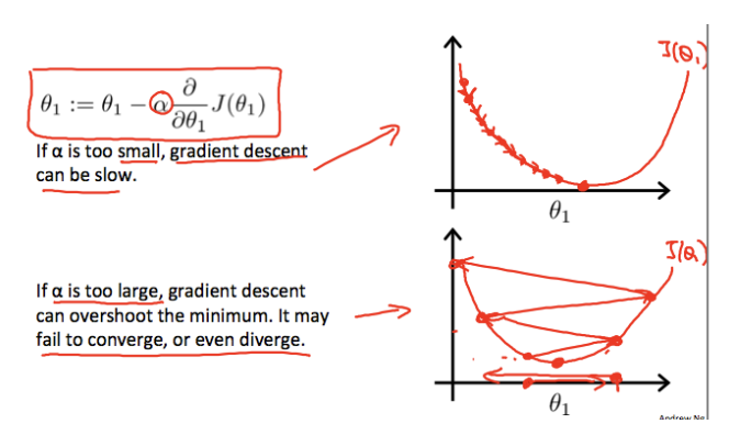
- $\alpha$ is the learning rate, controlling the step size. Too small slows convergence, while too large can overshoot the minimum
The gradient points in the direction of steepest increase in the cost function. Moving in the opposite direction reduces the mean squared error.
The effect of the learning rate is illustrated in the image below, using one feature ($\theta_1$) and the intercept ($\theta_0$). Each star represents a step, and the arrows indicate the direction toward the minimum. The path depends on the starting point and the learning rate, but for convex quadratic cost functions, the final solution is always the same.
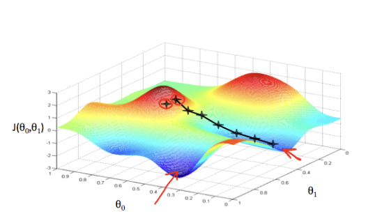
Source: Supervised Machine Learning: Regression and Classification
Because the squared error in OLS is quadratic, there is only one global minimum. Gradient Descent will always converge to this solution, although the exact path depends on the learning rate and stopping criteria.
Source: Supervised Machine Learning: Regression and Classification
Stochastic Gradient Descent (SGD)
Instead of computing the gradient over the entire dataset, SGD updates the coefficients using one random sample at a time. This reduces memory usage and speeds up per-iteration updates, but can cause noisy updates that oscillate around the minimum.
Stochastic Average Gradient (SAGA)
SAGA improves on SGD by storing an average of past gradients to reduce variance, leading to faster convergence. It is particularly efficient for sparse data or L1-regularised problems.
Coordinate Descent
Coordinate descent updates one coefficient at a time while holding the others fixed. This method is the default for Lasso and ElasticNet in Python’s scikit-learn and can handle large, sparse datasets efficiently:
$\theta_j := \theta_j - \alpha \frac{\partial J(\theta)}{\partial \theta_j}$
Regularisation
When using Ridge (L2), Lasso (L1), or ElasticNet penalties, the cost function becomes:
- Ridge: $J(\theta) = \frac{1}{m} \sum_{i=1}^{m} (y_i - x_i \cdot \theta)^2 + \lambda \sum_{j=1}^{n} \theta_j^2$
- Lasso: $J(\theta) = \frac{1}{m} \sum_{i=1}^{m} (y_i - x_i \cdot \theta)^2 + \lambda \sum_{j=1}^{n} |\theta_j|$
- ElasticNet: $J(\theta) = \frac{1}{m} \sum_{i=1}^{m} (y_i - x_i \cdot \theta)^2 + \lambda_1 \sum_{j=1}^{n} |\theta_j| + \lambda_2 \sum_{j=1}^{n} \theta_j^2$
Gradient descent can be used for Ridge regression, while coordinate descent is preferred for Lasso and ElasticNet, which is the default in Python’s scikit-learn. These methods iteratively update coefficients until convergence, automatically handling the regularisation penalties during each step.
OLS Assumptions
Regardless of how it’s fit, OLS relies on several key assumptions. These can be grouped into two main categories:
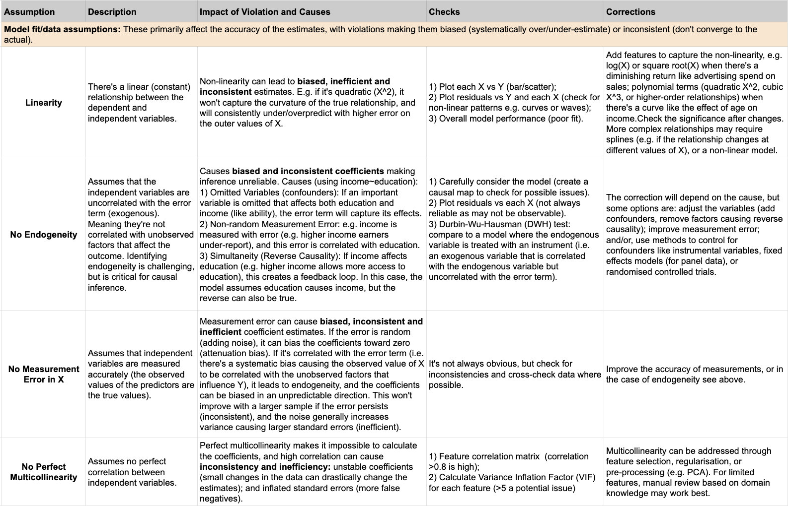
- 1) Model fit and data assumptions (linearity, no perfect multicollinearity, no endogeneity, no measurement error): These primarily affect the accuracy of the estimates themselves, making coefficients and predictions potentially biased (systematically over- or under-estimated) and inconsistent (not converging to true values even with larger samples). Violations of these assumptions lead to incorrect relationships being modeled, resulting in the estimates being systematically off.
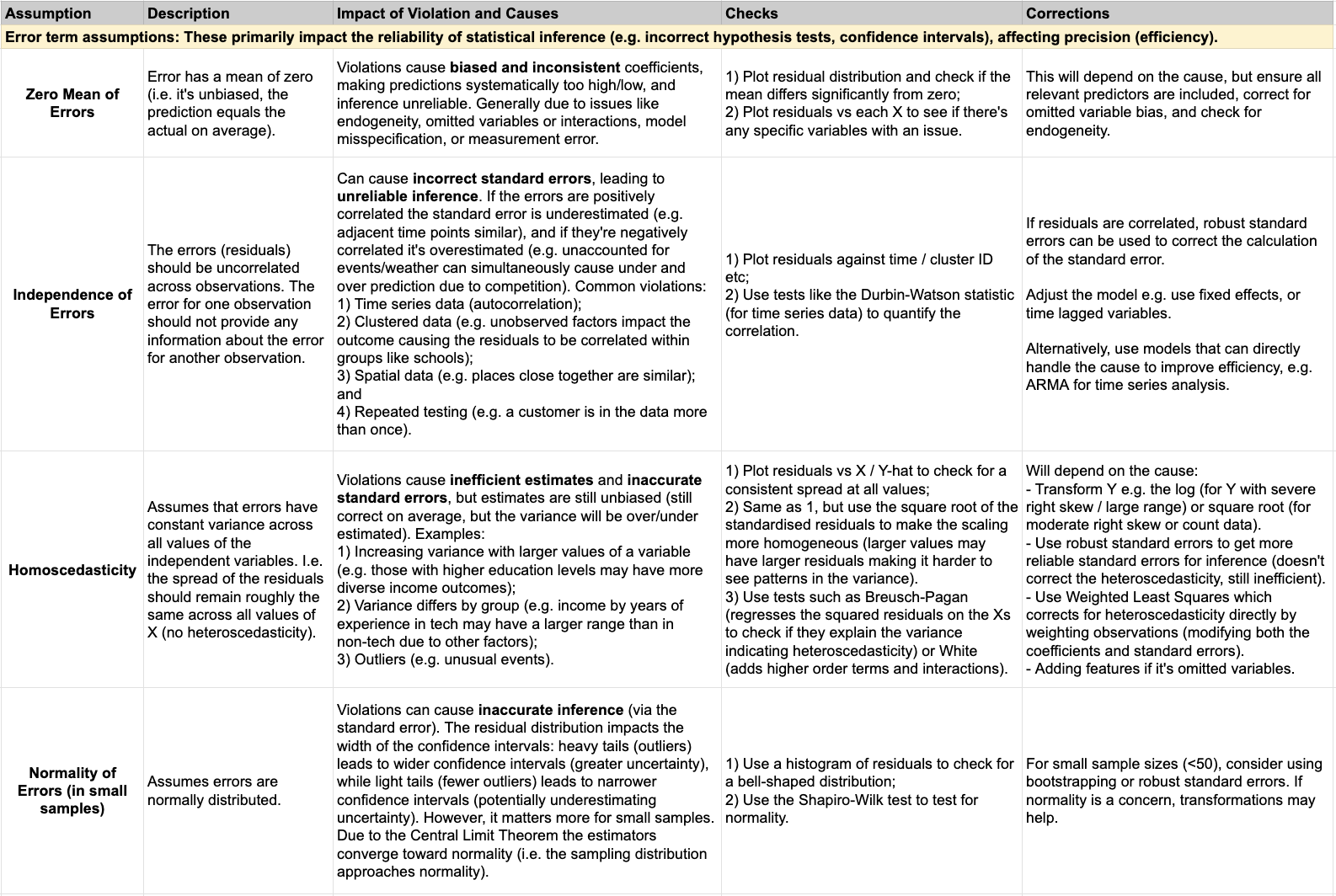
- 2) Error term assumptions (zero mean, independence, homoscedasticity, normality): These primarily impact the reliability of statistical inference, such as hypothesis tests and confidence intervals. Violations of these assumptions affect precision (efficiency), leading to inefficient estimates (larger standard errors and wider confidence intervals), though they may not necessarily cause bias in the coefficients themselves. In other words, the estimates might still be unbiased but less precise.
Below is a more detailed summary of each assumption, how to assess it, and how to potentially correct it:
Causal map
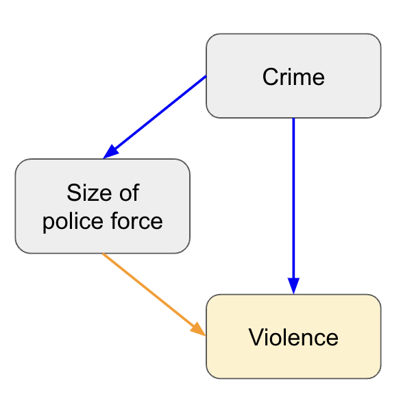
This is touched on under the no endogeneity assumption, but at the very start it can be useful to draw a causal map of all the features and how they are related to each other and the outcome (including those you don’t have). This can be as simple as writing down the outcome, then adding the common factors (features) that might influence it, with lines and arrows to show the expected relationship. Next you can add unmeasured (or difficult to measure) factors that might influence either the outcome or features. This process helps you understand how much of the outcome you are likely to be able to explain, allows you to be explicit in your assumptions, and can help you with interpreting the results. Using a very simplified example, if you predicted the rates of violence based on the size of the police force, you may conclude they’re positively correlated (more police equals more violence) because you’re missing the confounder of crime rate (higher crime equals more police and more violence).
This is also a good checkpoint to consider whether this is a problem you should proceed with. Given the potential outcomes, what actions can you take? Are the features things you can change or influence? What would your stakeholder do if the result is that X, Y, Z are influential. Are you framing this problem correctly, does it address the real question?
Evaluating the model
When evaluating the model, we want to assess whether we have a “good” model, meaning it fits the training data well, has good predictive accuracy (on unseen test data), and doesn’t violate the assumptions. This section will cover the most common metrics and plots, but you may need a deeper dive depending on your situation (e.g. if you suspect an assumption violation).
Split the data
To assess the predictive accuracy on unseen data you typically set aside some of your observations before you start the modelling process. This can be a fixed split (e.g. 80% used for training, 20% held out for testing), or you can use k-fold cross validation (train on k-1 folds and test on the remaining, repeating k times). The benefit of the cross validation approach being that we can use all of the data for training (more efficient), and we’re less likely to overfit as we’re splitting multiple times and averaging over these to understand the performance. However, it’s more computationally expensive, so better for smaller data sets (k is typically 5-10, but stability and cost increase with k).
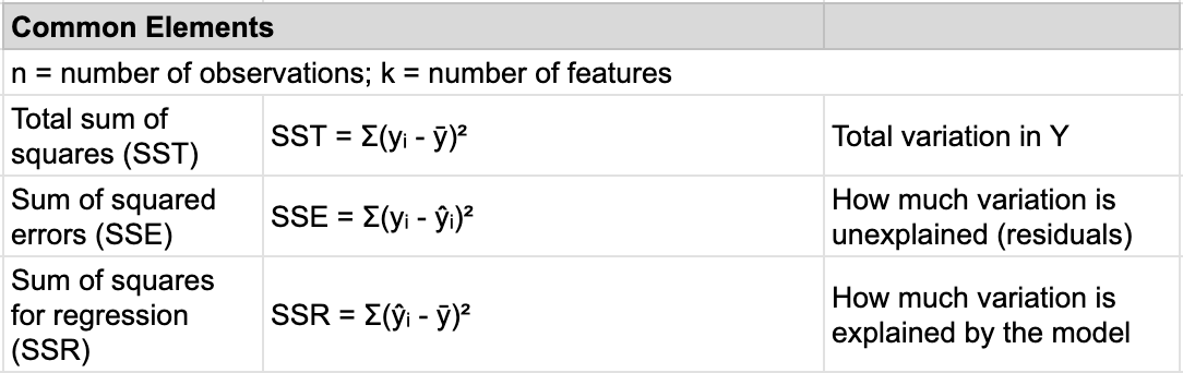
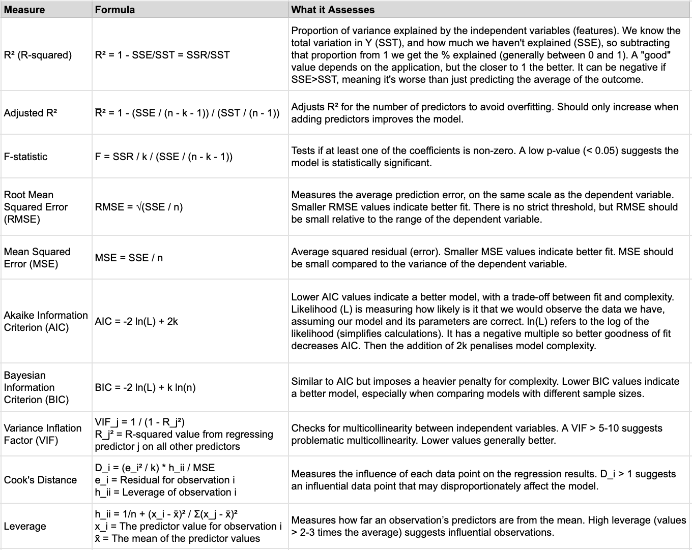
Metrics
Below are the most common metrics you’ll compute. The performance metrics (R², MSE, RMSE) are used to assess the model fit and generalisation, so we calculate them for both the training and test data and compare. If there’s overfitting we would see a divergence between the train and test results. For example, the training MSE would continue to decrease as complexity increases (more features), but the test MSE would start increasing as the model overfits the training data (starts finding patterns that don’t exist more generally). The diagnostic metrics (AIC, BIC, VIF, Cook’s Distance, and Leverage) would primarily be used on the training data as we’re trying to understand how the model fits the data and whether there are any violations of the assumptions.
An important distinction to make is whether your primary goal is to make a prediction, or to interpret associations. If you want to apply some treatment/change/action to new cases/customers based on the predicted outcome, then you have a prediction problem and will focus more on the performance metrics. If you’re primarily interested in understanding past outcomes, and what features were most important in deciding the outcome, then you have an interpretation problem and may be ok with lower performance metrics so long as you accurately capture the relationships of interest.
Residual Plots
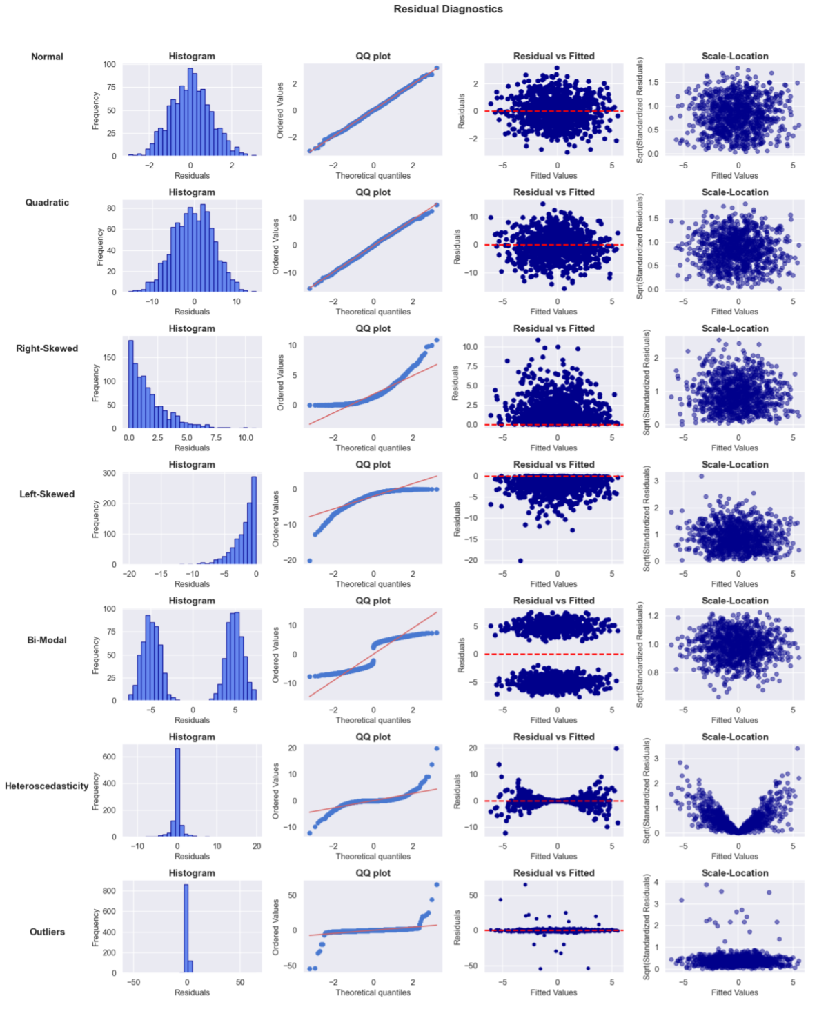
The most common residual diagnostic plots are:
- Histogram of Residuals: Distribution of residuals. Residuals should be approximately normally distributed and centered on zero. Non-normality is less of an issue for inference on large samples, but outliers, skewness, and patterns in the residuals still warrant attention. For example, skewness or heavy tails may indicate issues like omitted variables or model misspecification. If they’re not centered on zero, this would result in biased predictions (systematically off).
- QQ Plot (Quantile-Quantile Plot): Compares the distribution of residuals to a theoretical normal distribution. The x-axis is the quantiles of the standard normal distribution (e.g. the 1st, 5th, 10th, 50th, 90th, 95th, and 99th percentiles of a normal distribution, and so on), and the y-axis is the quantiles of the residuals from the actual model (sorted in ascending order). If the residuals follow a normal distribution, the points on the QQ plot should approximately follow the diagonal line. Deviations suggest non-normality, e.g. if the points in the tails deviate significantly (forming a curve), the residuals have heavier tails than a normal distribution (i.e., outliers are more common than expected); if the points curve away from the line in a consistent pattern (e.g. if the points are above the line on the left and below on the right), this suggests that the residuals may be skewed. Right skewness would cause the residuals to be more concentrated on the negative side, while left skewness would concentrate them on the positive side.
- Residual vs Fitted (predicted values) Plot: Used to check for non-linearity, unequal variance (heteroscedasticity), and outliers. Residuals should be randomly scattered around the zero line with no patterns or outliers. For example: patterns like a U-shape indicates the model might be missing an important non-linear relationship; if the spread is increasing/decreasing (like a fan), the variance of residuals is not constant across all levels of the predicted values (heteroscedasticity).
- Scale-Location Plot (or Spread-Location Plot): Specifically focuses on heteroscedasticity by displaying the spread of residuals across fitted values, using the square root of standardized residuals on the y-axis. This helps make the variance of residuals more comparable across the range of fitted values. The square root helps stabilize the variance and makes deviations from constant variance more apparent. Points should be evenly spread along the y-axis. A trend (e.g. increasing or decreasing spread) indicates heteroscedasticity, where variance of residuals is not constant.
- Residual vs X Plot: Used to check for non-linearity, unequal variance (heteroscedasticity), and endogeneity. Residuals should be randomly scattered around the zero line with no patterns or outliers. For example: patterns like a U-shape indicates the model might be missing an important non-linear relationship; if the spread is increasing/decreasing (like a fan), the variance of residuals is not constant across all levels of the predicted values (heteroscedasticity).
Below are some examples of how the plots might look for well behaved (normal) residuals (row 1) vs with different issues. Starting with the histogram and QQ plots, which assess whether residuals follow a normal distribution. In the normal example, the residuals are bell shaped and roughly follow the line in the QQ plot, supporting the normality assumption. However, in the quadratic example, the residuals show a slight curve at the extreme, suggesting the model isn’t capturing the non-linear relationship. The right-skewed and left-skewed examples reveal asymmetric distributions in the residuals, indicating potential model issues like omitted variables or incorrect transformations. The Residual vs Fitted plot helps detect heteroscedasticity, where the variance of residuals changes with fitted values; in the heteroscedasticity example, the spread of residuals increases, signaling a violation of constant variance. The Scale-Location plot further examines the spread of residuals. In the outlier example, we see large deviations, which could be due to influential data points. The bimodal example highlights a multi-modal distribution of residuals, suggesting that the model may be missing important factors.
Iterating on the model
Based on the above evaluation you’ll likely identify some possible improvements or issues that need to be resolved in a new iteration of the model. Below I’ll cover some of the topics that come up at this stage: outliers; standardising features; adding features; and, feature selection.
Handling outliers
Outliers are typically identified during the residual diagnostics, but can be more formally defined using Cook’s distance or leverage. You can remove the outliers (if erroneous, e.g. entry error), cap/winsorize the values (e.g. at the 5/95th percentile), or replace them with the mean. Whichever method you use, investigate a bit first to figure out the cause of the outlier, as they can reflect genuine phenomena in the data which you don’t want to remove. For example, travel agents might look like outlier customers in hotel bookings data. They likely behave differently so it might be better to model them separately or use interaction terms. In general, splitting the data into separate models for businesses and individuals is likely the most straightforward and interpretable solution, especially if the customer types have fundamentally different behaviors. However, if you want to keep everything in one model, consider using interaction terms to account for the different patterns and the outliers. For cases where the outliers are more random, capping is a simple, fast, and effective option to limit extreme values. However, there is data loss and it can introduce bias if the wrong thresholds are chosen. An alternative option is using a robust regression method (covered later), which modifies the model instead.
Standardised features
If you want to compare the coefficients, then it’s useful to put them all on the same scale by standardising the values before fitting the model (i.e. x - mean / std deviation). Then they can be ranked based on their absolute magnitude to understand which features have the largest effect on the outcome. Just keep in mind there’s still the issue of whether the coefficients are unbiased, and you’ll want to only consider those that are significant (covered later).
Adding more features
Adding new features that are predictive of the outcome can improve the model’s accuracy, but also the precision of the coefficient estimates (i.e. smaller confidence intervals). When the residual variance is reduced (reducing the unexplained variance), the standard errors of the coefficients are also reduced, leading to smaller confidence intervals. However, adding too many features that have a weak or no effect on the outcome leads to overfitting. If they’re highly correlated (multicollinearity), it can also destabilise the coefficient estimates and increase their variance. An example of this is adding features that are predictive of another feature, but not the outcome. It can lead to multicollinearity, or reduce the variance of the feature (which is harmful).
The other type of features you might add are variations of the existing, such as: polynomials (i.e. X^n to capture non-linearity); and, interactions (when the effect of one feature might depend on the value of a second feature). As with the above, adding too many can lead to overfitting. This is where the next section on feature selection is useful.
Feature Selection
If multicollinearity is an issue, a common solution is to reduce the feature set. However, in general a simpler model with fewer features is more desirable in terms of efficiency, interpretability, and performance (reducing risk of overfitting). It can be done in a few ways: stepwise selection (forward/backward/bi-directional); regularisation of the coefficients (lasso/ridge/elastic net); Principal Components Analysis (PCA); or, Partial Least Squares. Each has pros and cons, so it will depend on your problem and goals. However, a caution: automated feature selection is usually not recommended for causal inference, because a feature’s predictive power does not reliably indicate whether it is a confounder that must be adjusted for. It may still be useful as an exploratory tool to understand correlated features, but final feature selection should be guided by domain knowledge and the causal structure of the problem.
1. Stepwise selection
Stepwise selection involves iteratively fitting models with more/less features and checking some criterion to decide if the model performance is still improving beyond some threshold (e.g. AIC/BIC, adjusted \(R^2\)). These are easy to understand methods, but they’re computationally expensive (fitting many models), and can give inconsistent selections (sensitive to changes in data, may overfit the training data, depend on the starting point of forwards/backwards, and struggle with correlated features). For correlated features they might pick one over the other (when both are equally important), or include both when they’re redundant. This is particularly an issue if we are using the model to understand which features are most important.
Forward (iteratively add)
Fit a model with each individual feature (one by one) to get a measure of their significance (p-value, \(R^2\), AIC or BIC), then rank them based on this. Start with an empty model (no features, just intercept), then re-fit adding the most significant feature (e.g. has the lowest p-value), repeating the process adding one feature at a time until it doesn’t improve the model.
Backward (iteratively remove)
Start with all features in the model. Iteratively remove the least significant feature (e.g. highest p-value), each time re-fitting and calculating the significance of each feature. Stop when there are no insignificant features left, or when removing the feature worsens the model performance.
Bi-directional (combination)
Start with an empty model (intercept only), then add the most significant feature as in forward selection. After each step of adding features, check the signficance of the remaining features and remove any that are not signficant. Continue iterating, adding or removing features based on their significance until the model stabilises (no further improvement in the model performance). Note, this can also be done starting with the full set of features (as in backwards) and working that way.
2. Regularisation
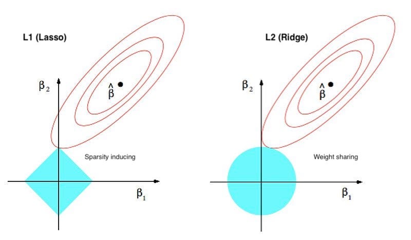
Regularisation methods add a penalty term to the loss function based on the coefficients, meaning they minimise both the RSS and the magnitude of the coefficients. Feature scaling (typically standardisation) is essential to avoid features with a larger range dominating the penalty term. The goal is to create a simpler model that generalizes well to unseen data. There’s a bias-variance trade-off here though, we sacrifice some accuracy on the training data (i.e. increase bias), to reduce variance and improve prediction accuracy on the test data. There are 3 main methods: 1) Lasso (L1) adds a penalty proportional to the absolute value of the coefficients (some go to exactly 0 as demonstrated below); 2) Ridge (L2) adds a penalty proportional to the square of the coefficients (shrinks all, but not to 0); and, 3) Elastic Net combines L1 and L2.
 Source: PennState Stat 897D
The strength of the regularisation is controlled by the parameter lambda (\(\lambda\)). Close to 0 (e.g. 0.01) there will be minimal regularisation (coefficients similar to without), around 1-5 there will be some shrinkage of the coefficients, and at large values (e.g. 10-100) there will be a lot of shrinkage and possibly all 0’s in the case of Lasso. Usually the value would be selected based on a grid search (test a set of values e.g. 0.001, 0.01, 0.1, 1, 10), potentially with cross-validation (to ensure generalises well).
Lasso (L1)
Lasso (Least Absolute Shrinkage and Selection Operator) penalises large coefficients by adding the sum of the absolute beta coefficients to the loss function (multiplied by the tuning parameter lambda). Using the absolute values leads to “corners” at zero (diamond or polygon shaped), so the optimization process will tend to set some coefficients to exactly zero, as this is the simplest and most efficient way to reduce the penalty. If there are highly correlated features, lasso tends to select one and shrink the others toward zero which can cause instability if features are highly correlated. If you use Lasso (or elastic net), you’ll need to fit the model using an iterative optimisation algorithm like Gradient Descent because Lasso reduces some coefficients to 0 (it becomes non-differentiable, meaning you can’t use simple calculus to find the optimal coefficients).
\[\text{Loss} = \text{RSS} + \lambda \sum_{j=1}^{p} |\beta_j|\]Where:
- RSS is the standard OLS loss: \(\sum_{i=1}^{n} \left( y_i - \hat{y}_i \right)^2\)
- \(\lambda\) is the regularisation parameter (lambda)
- \(\beta_j\) are the feature coefficients
- p is the number of features
If you’re interested in feature importance, you might consider using Lasso regularisation as a pre-processing step (remove the features that became 0). The coefficients after regularisation are biased (shrunk), so we then want to re-fit the model with the reduced feature set.
Ridge (L2)
Ridge penalises large coefficients by adding the sum of the squared coefficients. This will shrink coefficients, but not set them to 0 (optimal points are on a curve). Even in the case of highly correlated features, ridge tends to spread the shrinkage across all predictors. This makes it more stable than Lasso, reducing the variance. The normal equation can also be modified to add the penalty, meaning there is a single solution: (\(\mathbf{\beta}_{\text{ridge}} = \left( \mathbf{X}^T \mathbf{X} + \lambda \mathbf{I} \right)^{-1} \mathbf{X}^T \mathbf{y}\)).
\[\text{Loss} = \text{RSS} + \lambda \sum_{j=1}^{p} \beta_j^2\]Where:
- RSS is the standard OLS loss: \(\sum_{i=1}^{n} \left( y_i - \hat{y}_i \right)^2\)
- \(\lambda\) is the regularisation parameter (lambda)
- \(\beta_j\) are the feature coefficients
- p is the number of features
Elastic Net
Elastic net combines the Lasso and Ridge penalties to get the benefits of both, with an additional parameter (alpha) added to control the mix. It can be particularly useful for correlated features as the L1 component encourages the model to select a few important features (driving the irrelevant ones to zero), while the L2 component ensures that the remaining coefficients are regularized without being eliminated. For example, if two features are highly correlated, the L1 term will push both coefficients towards zero if both are irrelevant, but the L2 term ensures that they are shrunk together. If both are important, the model will keep them but shrink their coefficients. In this way it handles groups of features better, as correlated features are more likely to be selected or discarded together, rather than arbitrarily.
\[\text{Loss} = \text{RSS} + \lambda \left( \alpha \sum_{j=1}^{p} |\beta_j| + \frac{1 - \alpha}{2} \sum_{j=1}^{p} \beta_j^2 \right)\]Where:
- RSS is the standard OLS loss: \(\sum_{i=1}^{n} \left( y_i - \hat{y}_i \right)^2\)
- \(\lambda\) is the regularisation parameter (lambda)
- \(\beta_j\) are the feature coefficients
- p is the number of features
- \(\alpha\) is the mix of Lasso and Ridge (1 would be Lasso only, 0 would be Ridge only)
3. Principal Components (PCA)
Another solution is to replace the features with the first k components from a Principal Components Analysis. This is a dimensionality reduction technique that creates linear combinations of the features that are orthogonal to each other (independent). Imagine you have a cloud of data points in a high-dimensional space. PCA rotates and scales that cloud so that the “most informative” directions (those with the largest variance) become the new axes. Typically, you would choose how many components to keep based on how many are needed to explain “most” of the variance (e.g. 90 or 95%). For regression, you can also try different values and select k based on the test MSE. Two disadvantages of using PCA are: reduced interpretability (as each component is a mix of features); and, the components are selected without considering the relevance to Y (though generally if X is predictive of Y it will work well).
4. Partial Least Squares
Partial Least Squares (PLS) is another dimensionality reduction technique. Like PCA it creates linear combinations of the features (components) by projecting them onto a lower dimensional space. However, it searches for components that explain as much as possible of the covariance between X and Y, so it directly considers the relevance to Y in the process. Like PCA though, you still need to decide how many components to keep, and it can be hard to interpret if you want to understand the relationship of the original features with the outcome.
Statistical inference
When interpreting the coefficients, we typically have causal questions in mind (e.g. how does feature X affect Y?). In many cases we’ll only find what features are associated with the outcome. While it’s possible to use linear regression to get causal estimates (e.g. with data from a randomised trial), if we’re using observational data it’s very difficult to know if we’ve controlled for all confounders. However, it’s still a very useful technique for generating hypotheses that we can then try to validate with other methods. If your primary goal is prediction, then you may care less about the coefficients. However, it’s generally still useful, and in some cases required, to explain the predictions.
Coefficients
Let’s say we fit the following model:
\[Y_i = \beta_0 + \beta_1 X_{1i} + \beta_2 X_{2i} + \dots + \beta_k X_{ki} + \epsilon_i\]Where:
- \(Y_i\) is the outcome for observation i
- \(\beta_0\) is the intercept: a constant for Y when all X = 0
- \(\beta_1, \dots,\beta_k\) are the slope coefficients for the features \(X_1, \dots,X_k\): how much Y is expected the change for a one-unit change in \(X_k\), holding all other features constant (for binary, it’s the change from 0 to 1).
- \(\epsilon_i\) is the error (factors not in the model), estimated by the residual (actual-predicted value)
In general, the coefficients represent the effect of a one unit change in the feature on the outcome. However, interpreting the estimated coefficients (\(\hat{\beta_k}\)) depends on the feature types, so let’s work through some examples:
Binary and continuous features
\(Income_i = 30 + 5*Gender + 2*Experience\)
- Gender is coded 1=Male and 0=Female, all values in ‘000’s
- The intercept tells us that income is 30K on average when Gender=Female and Experience=0 (may be rare or non-existent).
- \(\hat{\beta}_1\)=5K tells us being male is associated with +5K in income (vs females), holding experience constant.
- \(\hat{\beta}_2\)=2K tells us every +1 year in experience is associated with +2K in income, holding gender constant.
- The predicted income for a female with 10 years experience is 30K + 5(0) + 2(10) = 50K, and for a male it would be 30K + 5(1) + 2(10) = 55K.
Interaction term
\(Income_i = 30 + 5*Gender + 2*Experience + 500(Gender*Experience)\)
- The intercept is unchanged.
- \(\hat{\beta}_1\)=5K tells us the difference in female and male income for individuals with 0 years experience (males earn 5K more).
- \(\hat{\beta}_2\)=2K tells us each year of experience is expected to add +2K when gender=0 (i.e. for females).
- \(\hat{\beta}_3\)=500 modifies the effect of experience for males: for males, each additional year of experience adds an extra +500 in income (on top of the 2K from \(\hat{\beta}_2\)).
- The predicted income for a female with 10 years experience would be: 30K + 5(0) + 2(10) + 500(0x10) = 50K.
- The predicted income for a male with 10 years experience would be: 30K + 5(1) + 2(10) + 500(1x10) = 60K.
- The difference boils down to \(\beta_1\) + \(experience * \beta_3\)
Quadratic term
\(Income_i = 30 + 5*Gender + 1*Age + -0.01*Age^2\)
- The intercept is unchanged.
- \(\hat{\beta}_1\)=5K tells us the difference in female and male income, holding age constant (males expected to have +5K).
- \(\hat{\beta}_2\)=1K tells us we expect +1K income for every additional year of age at the younger ages (before taking into account the quadratic effect), holding gender constant.
- \(\hat{\beta}_3\)=-0.01K=-10 tells us the rate at which income increases, decreases with age and eventually reverses (concave).
- The predicted income for a 30 year old male would be: 30 + 5(1) + 1(30) - 0.01(30^2) = 65 - 9 = 56K
- The predicted income for a 75 year old male would be: 30 + 5(1) + 1(75) - 0.01(75^2) = 110 - 56 = 54K
Adding higher order polynomials is the same, but capturing the higher order effects. E.g. Adding \(age^3\) to the above would capture the cubic effect of age on income, while the \(age^2\) still captures the quadratic effects, and age captures the linear.
Dummy variables
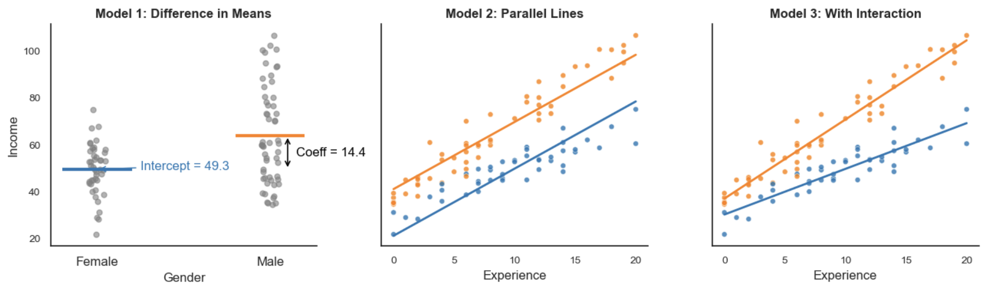
Let’s explore regression with dummy variables a little further. In a regression of an outcome on a dummy variable, the OLS estimator minimises the total squared error by choosing the group means as the best predictions. Suppose we model Income based on Gender, where Male = 1 and Female = 0:
\[Y_i = \beta_0 + \beta_1 \times \text{Gender}_i\]The intercept \(\beta_0\) is the mean of the baseline group (females), and the slope \(\beta_1\) is the difference in means between the two groups, which is the increment added to the intercept for males (\(\bar{x}_\text{males}-\bar{x}_\text{females}\)):
\[\beta_1 = \mathbb{E}[Y_i \mid \text{Gender}_i = 1] - \mathbb{E}[Y_i \mid \text{Gender}_i = 0]\]This happens because, mathematically, the value that minimises squared deviations from a set of numbers is their average, so the regression naturally aligns with the group means. If you were to minimise the absolute deviation, then it would be the median. Adding additional variables turns this into a conditional difference in means. For example:
\[Y_i = \beta_0 + \beta_1 \times \text{Gender}_i + \beta_2 \times \text{Experience}_i\]At every level of Experience, the predicted incomes for males and females are parallel lines. Gender shifts the intercept by a constant amount. This reflects the assumption that Gender and Experience affect Income independently. If we include an interaction term, the effect of Gender can vary with Experience:
\[Y_i = \beta_0 + \beta_1 \times \text{Gender}_i + \beta_2 \times \text{Experience}_i + \beta_3 \times (\text{Gender}_i \times \text{Experience}_i)\]With this, the predicted lines are no longer parallel, illustrating how Gender’s effect changes depending on Experience.
Categorical variables
Building on the previous discussion, we can fit a regression model where a categorical predictor with n categories is represented by k = n - 1 binary (dummy) variables. This approach estimates the average outcome for each category relative to a baseline group, rather than imposing a fixed functional form.For example, instead of assuming each additional year of experience adds a constant amount to income, we treat experience as a categorical variable with one dummy variable per year of experience (except the baseline):
\[\text{Income}_i = \beta_0 + \sum_{k=1}^{n-1} \beta_k \cdot D_{ik} + \varepsilon_i\]Where \(D_{ik}\) equals 1 if individual i belongs to experience category k, and 0 otherwise.
This model is fully saturated with respect to the categorical predictor, because it includes a distinct parameter for each category (except the baseline). It perfectly fits the training data by estimating the mean outcome for each category, minimizing residuals within groups and resulting in a residual sum of squares as low as possible given the data.
In this sense, the model is non-parametric: it does not assume any particular shape or linear relationship between experience and income. Instead, it allows the effect of experience on income to vary freely across categories, producing a stepwise function rather than a continuous slope.
The main advantage of doing this is flexibility: this model lets the data determine how income changes with experience without imposing linearity. However, this flexibility comes at a cost: higher variance in estimates, especially for categories with fewer observations, which can reduce precision and lead to overfitting.
Standard errors
The coefficient estimates are based on one sample, so like with all sample statistics we want to know how much these estimates might vary from sample to sample. The standard error is exactly this, it gives us a measure of the uncertainty of the estimate. This is then used to construct confidence intervals and do significance tests. The larger the standard error, the higher the uncertainty, and the wider the confidence intervals.
The standard error is the square root of the variance, calculated as follows:
\[SE(\hat{\beta}_j) = \sqrt{\text{Var}(\hat{\beta}_j)} = \sqrt{\hat{\sigma}^2 \left[ (\mathbf{X}^T \mathbf{X})^{-1} \right]_{jj}}\]We can break it down into a few steps:
1. Calculate the variance of the residuals (\(\hat{\sigma}^2\))
\(\hat{\sigma}^2\) is an estimate of the error term’s variance based on the residual variance (how spread out they are around the regression line):
\[\hat{\sigma}^2 = \frac{1}{n - k} \sum_{i=1}^{n} \hat{e}_i^2\]Where:
- \(\hat{e}_i = e_i - \hat{e}_i\), i.e. the residual for the i-th observation
- n is the number of observations (rows)
- k is the number of parameters (beta, including the intercept)
- n-k is the degrees of freedom
To get an unbiased estimate, we divide the sum of the squared residuals by the degrees of freedom instead of just n. This corrects for the fact k parameters were estimated (we’ve used up k pieces of information to estimate the parameters). If we divided by just n, we would bias the estimate downward (underestimate the true variance).
2. Calculate the Variance-Covariance Matrix
- We take our data matrix X (rows are observations, columns are features plus a column of 1s for the intercept).
- \(X^TX\): We transpose our matrix X (flip it), and then multiply with the original X matrix to get a square matrix. The diagonal is now the sum of the squared values for each feature (we’re multiplying the feature vector with itself, so the value in 1,1 is for X1, and 2,2 is for X2 and so on). This measures how much variation there is in each feature. The larger the number, the more information it provides to estimate the corresponding \(\beta\). The off-diagonal is the cross product of the feature pairs, capturing their covariance (how correlated they are, i.e. how much they move together). Highly correlated features would result in large numbers in the off-diagonal, and independent (orthogonal) features would result in zeros (though a 0 covariance doesn’t prove independence).
- \((X^TX)^-1\): The inverse of \(X^TX\) gives us the scaling factors that “remove” the dependencies between the features (recall a matrix multiplied by it’s inverse returns the identity matrix with 1s on diagonal, 0s off). Given the way we calculate the inverse, the diagonal is impacted by the off-diagonal. Stronger correlations (large off-diagonal values in \(X^TX\)) lead to larger diagonal values in \((X^TX)^-1\), indicating higher variance (uncertainty).
3. Take the diagonal element \(\left[ (\mathbf{X}^T \mathbf{X})^{-1} \right]_{jj}\)
Take the diagonal element of the inverse matrix \((X^TX)^-1\) corresponding to the coefficient \(\hat{\beta}_j\). This tells us how the feature corresponding to \(\hat{\beta}_j\) influences the variance of the coefficient estimate, accounting for the amount of variance in the feature and the correlation with other features. If the feature is poorly measured (e.g. it has low variance or is highly correlated with other features), the variance of the coefficient estimate \(\hat{\beta}_j\) will be large, indicating greater uncertainty about the estimate. If the feature has a lot of variance or is uncorrelated with the other features, then it’s the opposite and we have greater certainty and so a smaller \(\hat{\beta}_j\) variance.
4. Pull it back together
Now we have the components to calculate the variance of each \(\hat{\beta}_j\). Recall, the standard error tells us how much we expect \(\hat{\beta}_j\) to deviate from the true \(\beta_j\) on average due to sample variability. There are two sources of uncertainty here: variability in the error term which is the same for all coefficients and taken from step 1 (i.e. variability in the outcome unexplained by the model); and, variability in the features from step 3 (particular to feature j, \(\left[ (\mathbf{X}^T \mathbf{X})^{-1} \right]_{jj}\)):
\[\text{Var}(\hat{\beta}_j) = \hat{\sigma}^2 \left[ (\mathbf{X}^T \mathbf{X})^{-1} \right]_{jj}\]To put the variance back in the same units as \(\hat{\beta}_j\), the standard error takes the square root:
\[SE(\hat{\beta}_j) = \sqrt{\hat{\sigma}^2 \left[ (\mathbf{X}^T \mathbf{X})^{-1} \right]_{jj}}\]When a feature has a large variance and is uncorrelated with the other features, the coefficient has a smaller variance and thus smaller standard error (more precise estimate). If it is highly correlated with other features, the variance of the coefficient and thus standard error increases (harder to isolate the unique effect of that feature). This is the issue of multicollinearity, which can make the coefficients unstable or imprecise. As the sample size increases, both \(\hat{\sigma}^2\) and \((X^TX)^-1\) become more stable and the standard error decreases (more precise estimates).
Other formulas
You might also see a simplified version of the standard error formula, which doesn’t account for correlation between the features. In this case we just divide by the j-th diagonal element of \(X^TX\) (the sum of squared values for feature j), instead of multiplying by the diagonal of \((X^TX)^-1\):
\[\text{SE}(\hat{\beta}_j) = \sqrt{\frac{\hat{\sigma}^2}{\left( \mathbf{X}^T \mathbf{X} \right)_{jj}}}\]You may also see the non-matrix form with the sum of squared values in the denominator (equivelant to the diagonal of \(X^TX\)):
\[\text{SE}(\hat{\beta}_j) = \sqrt{\frac{\hat{\sigma}^2}{\sum_{i=1}^n x_{ij}^2}}\]If the features are not correlated, then these formulas would be suitable and don’t require calculating the inverse matrix.
Robust standard errors
The standard error depends on the variance of the error term, and so it’s accuracy depends on the assumptions of homoscedasticity (non constant error term variance could make them inflated/deflated) and independence of the errors (correlated residuals typically results in under-estimating the standard error). In both cases the coefficients may be unbiased, but the standard errors are unreliable (and thus hypothesis tests and confidence intervals will be unreliable). Robust standard errors are techniques that adjust the calculation of the standard errors to allow for these violations. They’re done after fitting the model, and only adjust the standard error, not the coefficient itself. Many of the common technqiques are sandwich estimators, meaning the estimator is “sandwiched” between two matrices: one accounting for the model fit (e.g. the covariance of the predictors), and the other accounting for the residuals or the variation in the error term. The first three below are examples of this. The exception is the fourth (bootstrapped standard errors), which use re-sampling instead.
1. White’s HSCE (heteroscedasticity-consistent standard errors)
This corrects for heteroscedasticity (non-constant variance in the residuals) by adjusting the calculation of the variance-covariance matrix. Instead of assuming the error variance is constant like above (\(\hat{\sigma}^2\) = the sum of squared residuals divided by dof), we allow the error variance to vary across the observations by creating a diagonal matrix of the squared residuals (i.e. an nxn matrix with the squared residuals on the diagonal and 0’s off). This is then used to calculate the variance:
\[\hat{V}_{\text{White}} = (X^T X)^{-1} X^T \hat{\Sigma} X (X^T X)^{-1}\] \[\hat{SE}(\hat{\beta}_j) = \sqrt{\hat{V}_{\text{White}, jj}}\]Where:
- The first \((X^T X)^{-1}\) scales the original covariance matrix of the coefficients in the absence of heteroscedasticity. It’s adjusting for the relationships between the independent variables like before.
- \(X^T \hat{\Sigma} X\) adjusts the covariance matrix for the varying error variances (heteroscedasticity) by incorporating the squared residuals (\(\hat{\Sigma}\) is the diagonal matrix of squared residuals)
- Then the second \((X^T X)^{-1}\) applies the same scaling to the adjusted covariance matrix.
For small samples, there’s also a variation called Huber-White Standard errors. It uses a squared residuals approach, similar to White’s method, but adds additional adjustments for more reliable estimates in small samples.
2. Clustered standard errors
This technique adjusts the variance co-variance matrix for within-cluster correlation of the errors by summing the contributions of each cluster’s residuals. Correlated errors is a common issue in grouped data due to shared unobserved factors within a group (e.g. same school, city/region). It still assumes the errors are independent between groups (e.g. two students in different schools shouldn’t have correlated residuals). Similar to White’s, we use a diagonal matrix of squared residuals to allow for heteroscedasticity, but now they are cluster specific (\(\hat{\Sigma}_c\) is calculated for each cluster c) and then summed to produce an overall estimate of the covariance between the features and the residuals:
\[\hat{V}_{\text{clustered}} = (X^T X)^{-1} \left( \sum_{c=1}^{C} X_c^T \hat{\Sigma}_c X_c \right) (X^T X)^{-1}\] \[\hat{\text{SE}}_{\text{clustered}}(\hat{\beta}_j) = \sqrt{\left[ \hat{V}_{\text{clustered}} \right]_{jj}}\]3. Newey-West
Newey-West standard errors are for time series data when there is both heteroscedasticity and autocorrelation (errors in one time period may be correlated with errors in previous or future periods, also called serial correlation). It adjusts the variance-covariance matrix to consider lags of residuals (addressing autocorrelation), and allows the error variance to differ across observations (addressing heteroscedasticity). For smaller samples (<50), fewer lags can be included so bootstrapping might be more robust (see next section).
\[\hat{V}_{\text{NW}} = (X^T X)^{-1} \left( \sum_{t=1}^{n} \hat{\epsilon}_t^2 X_t X_t^T + \sum_{q=1}^{Q} \left( \sum_{t=q+1}^{n} \hat{\epsilon}_t \hat{\epsilon}_{t-q} X_t X_{t-q}^T \right) \right) (X^T X)^{-1}\]Where:
- X is the nxk matrix of features (n rows for n time periods)
- \(\hat{\epsilon}_t = Y_t - X_t \hat{\beta}\) is the residual at time t
- \(X_t\) is the row vector of features for observation t
- Q is the number of lags to include for past residuals, with larger values capturing more long term autocorrelation at the cost of efficiency. A rough rule is to start with \(Q \approx \sqrt{n}\).
- The first term \(\sum_{t=1}^{n} \hat{\epsilon}_t^2 X_t X_t^T\) adjusts for heteroscedasticity, just like White’s robust standard errors scaling the rows of X by the squared residuals at the time.
- The second term \(\sum_{q=1}^{Q} \left( \sum_{t=q+1}^{n} \hat{\epsilon}_t \hat{\epsilon}_{t-q} X_t X_{t-q}^T \right)\) adjusts for serial correlation by incorporating the residuals at time t and t-q, scaled by the corresponding features. This is summed across the Q lags.
- These are sandwiched by \((X^T X)^{-1}\) to account for the variance of the estimated coefficients.
4. Bootstrapped standard errors
Bootstrapped standard errors are a non-parametric way to estimate the variability. Given it doesn’t rely on any distributional assumptions about the errors, it can handle heteroscedasticity, autocorrelation, and non-normality of errors. It involves repeatedly drawing random samples with replacement of size n from the original data. Then for each sample, you re-fit the OLS, and estimate the coefficients. The idea is to approximate the sampling distribution of each coefficient. The standard deviation of these estimates gives us our bootstrapped standard error:
\[\text{SE}_{\beta_j}^{\text{bootstrap}} = \sqrt{\frac{1}{B} \sum_{b=1}^{B} \left( \hat{\beta}_{j,b}^* - \hat{\beta}_j \right)^2}\]Where:
- B is the number of bootstrap resamples
- \(\hat{\beta}_{j,b}^*\) is the estimated coefficient from the b-th bootstrap sample
It can work even in small samples, but is computationally expensive as n and the number of samples increases.
Confidence Intervals (CI)
Recall, a confidence interval quantifies the uncertainty of a sample estimate (in this case \(\hat{\beta}_j\)), by giving us a range of values around the estimate that “generally” contains the true population value. Like any sample estimate, it’s unlikely our coefficient is exactly equal to the true value. If we repeatedly sampled, we would get a distribution of coefficients around the true value (a sampling distribution), that with a large enough n converges to the normal distribution. Therefore, we can use the t distribution in it’s place, which has heavier tails for smaller samples, but converges to normal as n increases. Using the standardised t distribution (centered on 0, units are standard errors), we can pick how many standard errors we need to get x% coverage of the samples. Or in other words, how many standard errors will ensure that x% of samples contain the true value. This becomes the “critical value” that we multiply our standard error with to get the confidence interval:
\[\hat{\beta}_j \pm t_{\frac{\alpha}{2}, \, df} \cdot \text{SE}(\hat{\beta}_j)\]Where:
- \(\hat{\beta}_j\) is the estimated coefficient for feature j
- \(t_{\frac{\alpha}{2}, \, df}\) is the critical t-value for the desired confidence level, with df degrees of freedom.
- \(\text{SE}(\hat{\beta}_j)\) is the standard error, as calculated in the above section
To determine the critical value, we have to decide the confidence level (1-alpha). Typically in a business context the confidence is set at 95% (alpa=0.05) or 90% (alpha=0.1). The higher the confidence required, the wider the confidence interval will be to increase the chances of capturing the population value. Noting, the actual value may or may not be in the range for our given sample. Coming back to the sampling distribution (distribution of coefficient estimates across multiple samples), if we placed the resulting distance around each estimate we would see that 95% of the time (for alpha=0.05) the true value is within the interval. The other 5% of the time, we have a particularly high or low estimate (by chance) and miss the actual value.
You can read more on confidence intervals here.
Hypothesis tests
As we covered above, we’re estimating these coefficients based on just one sample. It’s possible that even if there is no relationship between feature j and the outcome y, we get a non-zero coefficient in our model. Hypothesis testing tells us how often we would expect to see a coefficient as large as that observed (or larger), when there’s actually no effect. If it’s uncommon, then we conclude there is likely a real effect. There are two main types of hypothesis tests we’re interested in here: 1) a t-test on the individual coefficients to determine if the effect of feature j on the outcome is statistically significant; 2) an F-test on all the coefficients at once to determine if they have an effect on the outcome (i.e. not likely that all are 0).
1. Individual coefficients (t-test)
This uses the t-distribution, so if the confidence interval contains 0, the result will be not-significant (assuming the same alpha is used etc). Let’s work through the process:
Null hypothesis (\(H_0: \beta_j = 0\)): feature j has no effect on the outcome y.
Alternate hypothesis (\(H_0: \beta_j \neq 0\)): feature j has some non-zero effect on the outcome y.
- t-statistic for the coefficient: \(t_j = \frac{\hat{\beta}_j}{\text{SE}(\hat{\beta}_j)}\)
- Degrees of freedom = n-k (observations - number of beta coefficients incl. intercept)
- Alpha (\(\alpha\)): commonly 0.05 (95% confidence) or 0.1 (90% confidence).
- Critical t: The value of the t-distribution that leaves \(\alpha / 2\) in each tail of the distribution (or just \(\alpha\) for a one sided test). This depends on the degrees of freedom, as it defines the shape of the t-distribution. We can find the critical t value using the cumulative distribution function to measure the area under the curve, but there are also pre-computed reference tables. This is then compared with the t-statistic. If the absolute t-statistic exceeds the critical t-value, then we reject the null hypothesis. It’s uncommon we would see a \(\beta_J\) this large by chance.
- P-value: This is the area under the curve on the t-distribution beyond the observed absolute t-statistic for the coefficient (i.e. how often we see samples with values greater than or equal to this). We double it for a 2-sided test as we’re considering both sides. If the p-value is less than or equal to our chosen alpha, we reject the null hypothesis (it’s uncommon we would see a \(\beta_J\) this large by chance). If it’s greater than alpha, we can’t reject the null.
Hopefully, you can see the p-value and the test statistic will result in the same conclusion as they’re using the same cutoff point (based on the alpha and degrees of freedom). The larger the absolute value of the t-statistic, the smaller the p-value will be and vice versa. For more on p-values, read this.
2. All coefficients vs intercept only (F-test)
To test the joint significance of multiple features we can use an F-test. The hypothesis becomes:
\[H_0: \beta_1 = \beta_2 = \dots = \beta_k = 0\] \[H_1: \text{At least one } \beta_i \neq 0 \quad \text{for some } i \in \{1, 2, \dots, k\}\]To assess this, we compute the F-statistic which is the ratio of explained (average per feature) and unexplained variance. This can also be though of as comparing the “full” model (all features) to an intercept only model (just the average and residuals). Like with the t-test, we compare the F statistic to the critical value from the F-distribution, based on the alpha and degrees of freedom of the numerator and denominator. The F distribution is a ratio of two independent chi-squared distributions, so it’s right skewed, but approaches normal as the degrees of freedom increase in both the numerator and denominator.
\[SSR = \sum_{i=1}^{n} (\hat{y}_i - \bar{y})^2\] \[SSE = \sum_{i=1}^{n} (y_i - \hat{y}_i)^2\] \[F-statistic = \frac{MSR}{MSE} = \frac{\frac{SSR}{k}}{\frac{SSE}{n - k - 1}}\]Where:
- SSR is the portion of total variation in y which is explained by the features. Mean Square for Regression (MSR) divides this by k to get the average per feature.
- SSE is the portion of total variation in y that is not explained by the model (i.e., the residual variation). Mean Square for Error (MSE) divides this by the degrees of freedom (independent observations remaining to estimate the unexplained variation).
- k is the number of features (excl. intercept as it doesn’t explain variance in y)
- n is the number of observations
- The degrees of freedom is k for the numerator, n-k-1 for the denominator
If F is large and we exceed the critical F value (the explained variance is much greater than the unexplained), we reject the null and conclude at least one of the features is significantly related to the outcome (as the features collectively explain a significant portion of the variation in the outcome). The model as whole is a good fit. If F is small and it doesn’t exceed the critical F threshold, the features don’t explain much variation, and the model may not be useful (fail to reject H0).
3. Nested models (F-test)
The F-test can also be used to compare models where one uses a subset of the features of the other. For example, maybe we want to see if a simpler model (let’s call this model 1) with fewer features is just as good in terms of variance explained as the more complex model (model 2).
\(H_0: \beta_n = 0\) (for the fuller model 2, i.e. the additional features don’t explain any additional variance in the outcome)
\(H_1: \beta_n \neq 0\) (the additional features do explain additional variance in the outcome)
To calculate F we would fit both models and calculate the SSE and SSR for each as above, then F is as follows:
\[F = \frac{(SSR_2 - SSR_1) / (p_2 - p_1)}{SSE_2 / (n - p_2)}\]Where:
- \(SSR_2 - SSR_1\) is the additional variance explained by the fuller model, and dividing by \(p_2 - p_1\) makes it the average per additional feature
- The denominator is the mean square error (MSE) for the more complex model
This is very similar to the F-test described above, but now we’re looking at the ratio of the additional explained variance in model 2 (per additional feature) and the unexplained variance in model 2. When finding the critical F value, the degrees of freedom also differ and will be \(p_2-p_1\) (diff in nr of features) for the numerator, and \(n - p_2\) (total observations minus the number of features) for the denominator. If F is large and significant, the additional features significantly improve the model and we should prefer the more complex model.
Extensions
Weighted Least Squares (WLS)
This is a variation of OLS that can handle heteroscedasticity (when error terms have non-constant variance). When there’s heteroscedasticity, the coefficient estimates remain unbiased but are no longer efficient (larger standard errors than necessary). This can lead to inefficient estimation and incorrect statistical inferences (such as unreliable confidence intervals or hypothesis tests). In WLS, instead of treating each observation equally, each observation is given a weight that reflects the level of uncertainty or variability in that particular observation (typically the inverse of the variance of the error term). The idea is to give more weight to observations that are more reliable (i.e., those with smaller variance) and less weight to observations that are less reliable (i.e., those with larger variance). Unlike robust standard errors which correct only the standard errors after fitting the OLS model, WLS adjusts the regression estimation process itself, adjusting the coefficients and their standard errors in one go. WLS is a better choice if you have reliable weights (i.e. a good reason to believe that some observations should be given more weight than others).
In WLS we minimize the weighted sum of squared residuals (WSS), rather than the usual sum of squared residuals (RSS):
\[\text{WSS} = \sum_{i=1}^n w_i (Y_i - \hat{Y}_i)^2\]Which gives us the following solution for the weighted least squares estimates:
\[\hat{\beta} = (X^T W X)^{-1} X^T W Y\]The weights are not typically known in advance, so a common approach is to run an OLS regression and use the squared residuals as estimates of the error variances (then taking the inverse as the weight):
\[w_i = \frac{1}{\sigma_i^2}\]For example, if you’re trying to predict income based on education across different regions, the variability in income could differ by region. Using WLS, you would give more weight to observations from regions where income variability is lower and less weight to regions with higher income variability to improve the efficiency of the estimates. However, it’s easy to see how this results in unequal treatment of certain groups, which makes interpretation more complex and can result in bias. For example, in this case the coefficients become biased toward low variance regions, and could be more or less significant under a different weighting. In other words, the results are not as generalisable, so depending on the purpose this might not be a good solution.
Generalized Least Squares (GLS):
GLS generalizes OLS to handle error structures with heteroscedasticity (non-constant variance) and autocorrelation (correlation between errors). It’s similar to WLS in that it explicitly adjusts the model to account for the error structure. However, it takes the weights from the inverse of the full error covariance matrix allowing for any general error covariance structure, whereas WLS uses the inverse of the error variances for each observation so is specifically for heteroscedasticity (assumes errors are uncorrelated). This makes it more flexible, but more computationally complex.
\[\hat{\beta}_{GLS} = \left(X^T \Sigma^{-1} X\right)^{-1} X^T \Sigma^{-1} Y\]Where:
- 𝑋 is the matrix of explanatory variables (independent variables),
- Y is the vector of dependent variables,
- β is the vector of regression coefficients,
- Σ is the covariance matrix of the error terms, which is often unknown and must be estimated.
GLS is used when you know or have a good estimate of the covariance structure of the errors and you want to correct the model itself to be more efficient. Robust standard errors make fewer assumptions than GLS, but the model itself is still inefficient. You would use robust standard errors instead when you’re concerned about the precision of the estimates, but not the model’s fit.
Generalized Linear Models (GLM)
Generalized Linear Models (GLM) are a more general framework that allow for different distributions for the dependent (outcome) variable (e.g. normal, binomial for binary, Poisson for count data, Gamma for positive continuous data with skewed distributions), and a range of link functions that connect the expected value of the dependent variable to the linear predictor (e.g. Identity for normal, Logit for binary, Log for Poisson, Inverse for Gamma). OLS is a specific case of GLM where the dependent variable follows a normal distribution, and the identity link function is used (i.e. the expected value of the outcome variable is a linear combination of the features). When the dependent variable is binary and the link is logit, this is Logistic Regression.
Maximum Likelihood Estimation (MLE)
Maximum Likelihood Estimation (MLE) is another more general framework that applies to a broader range of models and error distributions. MLE selects the parameters that make the observed data most probable, based on the likelihood function. Therefore, MLE will yield the same estimates as OLS when the error term is assumed to follow a normal distribution. This is because maximising the log-likelihood for normal errors results in the same objective function as OLS (the sum of squared residuals).
Robust regression
Robust regression methods reduce the influence of outliers on the model’s estimated coefficients, leading to more reliable results when there’s anomalies in the data. Some common examples include:
- Least Absolute Deviations (LAD) Regression: minimizes the sum of the absolute differences between the observed and predicted values (reducing the influence of large deviations). It’s a good simple approach when the data is small (requires iterative optimisation).
- Huber Regression: for smaller errors, it behaves like OLS, but for larger errors (which would normally be treated as outliers), it switches to absolute differences, reducing the impact of outliers. The tuning parameter (δ) must be selected, which defines the threshold where the loss function switches from quadratic to linear.
- RANSAC (Random Sample Consensus): The algorithm randomly selects a subset of the data, fits the model, and then checks how many of the remaining data points fit well with the model. It repeats this process many times and selects the model with the highest number of inliers. It works well when there’s a lot of outliers and can be used with large data sets, but is computationally expensive.
- Quantile Regression: estimates the conditional quantiles of the response variable (like the median or other quantiles) rather than the mean. It works well with skewed data and outliers, but is only suitable if you’re interested in estimating quantiles.
These methods don’t directly modify the data, instead adapting the model fitting process to down-weight the influence of outliers, which can lead to more reliable parameter estimates. Therefore, they may be more desirable than the methods for outliers discussed earlier which change the data instead of the model (e.g. removing / capping / replacing outliers). However, these methods are less efficient for normally distributed errors, are more complex, and generally more computationally expensive.
Summary
OLS is a simple, yet powerful technique for estimating the parameters of a linear regression model, but it relies on several assumptions. Other than misspecifications of the model (e.g. non-linear relationships, or omitted variables), the main limitation is it’s sensitivity to outliers. While it is widely used in practice due to its efficiency and ease of interpretation, it is important to check whether the assumptions hold to ensure valid and reliable results. More complex models may better fit the data in some cases (e.g. Random Forest or XGBoost), which can be combined with something like SHAP for interpretation. However, even then, if you’re working with observational data you should be cautious about making causal claims due to the potential for uncontrolled confounders. That said, it’s still a very useful method for generating hypotheses, which you can then use other methods to validate (e.g. randomised experiments).
References:
- For a more detailed refresher on Linear Algebra, Strang’s MIT course is very good. Note, there’s no need to scale the features when using the normal equation.
- Supervised Machine Learning: Regression and Classification course by Andrew Ng. This was helpful for understanding the Gradient Descent approach.
- Hastie, T., Tibshirani, R., & Friedman, J. H. (2009). The Elements of Statistical Learning: data mining, inference, and prediction. 2nd ed. New York, Springer. This is a great book and available for free download.